Page 137 - Air pollution and greenhouse gases from basic concepts to engineering applications for air emission control

4.5 Aerosol Particle Size Distribution 111

150000 150000
Number concentration of particles, #/cm3 100000 Number concentration of particles, #/cm3 100000

50000
50000

0 0
0 50 100 150 200 250 300 1 10 100 1000
dp (nm) dp (nm)

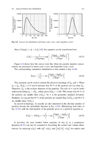
Fig. 4.4 Aerosol size distribution (left linear scale x-axis, right logarithm x-axis)

Since f logd p ¼ d p f ðd p Þ [9], the equation can be transformed into
2
" #
1

logd p logd pg
fd p ¼ p ffiffiffiffiffiffi exp p ffiffiffi ð4:53Þ
2pd p logr 2logr
Figure 4.4 shows how the curves look like when the particle number concen-
trations are presented in linear scale x-axis and logarithm scale x-axis.
The corresponding cumulative distribution is then similar to Eq. (4.49)

1 logd p logd pg
;ðd p Þ¼ 1 þ erf p ffiffiffi ð4:54Þ
2 2logr
This equation can be used to explain the physical meanings of d pg and r. When
d p ¼ d pg , ;ðd p Þ¼ 0:5 and it indicates that 50 % of the particles are less than d pg .
Therefore, d pg is the median diameter of the particles. The role of r can be better

understood letting d p ¼ rd pg , which gives ; d p ¼ 0:84: This means that 84 % of

the particles are smaller than rd pg .So r is the geometric standard deviation.

Similarly, we can get that 95 % of the particles are smaller than 2rd pg and 99.5 %

are smaller than 3rd pg .
In aerosol technology, we usually are also interested in the absolute number of
particles besides the probability function in Eq. (4.54). Multiplying both sides of
Eq. (4.54) with the total number of the particles gives us a practical equation as

logd p logd pg

Fd p ¼ N;ðd p Þ¼ N 1 þ erf p ffiffiffi ð4:55Þ
2logr
It describes the total number below particles of size d p in a population.
Equation (4.55) can also be extended to describing the surface and volume distri-

2 3
butions, by replacing nd p with pd nd p and pd =6 nd p for surface and
p p