Page 147 - Air pollution and greenhouse gases from basic concepts to engineering applications for air emission control

5.1 Adsorption 121

• The adsorbed layer is made up of a single layer of molecules.
• Adsorption is a reversible process.
• The process is dynamic: the adsorbed molecules do not move on the surface of
the adsorbent, but they may reenter the air stream.
• The enthalpy of adsorption is the same for all molecules independently of how
many have been adsorbed.
At equilibrium the number of molecules being adsorbed equals to the number of
molecules leaving the adsorbed state, i.e., Rate of adsorption = Rate of desorption

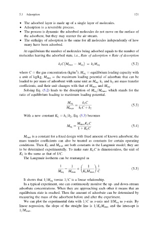
k 1 CM max M eq ¼ k 2 M eq ð5:2Þ
3
where C ¼ the gas concentration (kg/m ); M eq ¼ equilibrium loading capacity with
a unit of kg/kg, M max ¼ the maximum loading potential of adsorbate that can be
loaded to per mass of adsorbent with same unit as M eq .k 1 and k 2 are mass transfer
coefficients, and their unit changes with that of M max and M eq .
Solving Eq. (5.2) leads to the description of M eq =M max , which stands for the
ratio of equilibrium loading to maximum loading potential.

M eq k 1 C
¼ ð5:3Þ
M max k 1 C þ k 2

With a new constant K L ¼ k 1 =k 2 , Eq. (5.3) becomes
M max K L C
M eq ¼ ð5:4Þ
1 þ K L C

M max is a constant for a fixed design with fixed amount of known adsorbent; the
mass transfer coefficients can also be treated as constants for certain operating
conditions. Then K L and M max are both constants in the Langmuir model; they are
to be determined experimentally. To make sure K L C is dimensionless, the unit of
K L is the same as that of 1/C.
The Langmuir isotherm can be rearranged as

1 1 1 1
¼ þ ð5:5Þ
M eq M max K L M max C
It shows that 1=M eq versus 1=C is a linear relationship.
In a typical experiment, one can continuously monitor the up- and down-stream
adsorbate concentrations. When they are approaching each other it means that an
equilibrium state is reached. Then the amount of adsorbate can be determined by
measuring the mass of the adsorbent before and after the experiment.
We can plot the experimental data with 1=C as x-axis and 1/M eq as y-axis. By
linear regression, the slope of the straight line is 1=K L M max and the intercept is
1=M max .