Page 134 - Algorithm Collections for Digital Signal Processing Applications using MATLAB

122 Chapter 3

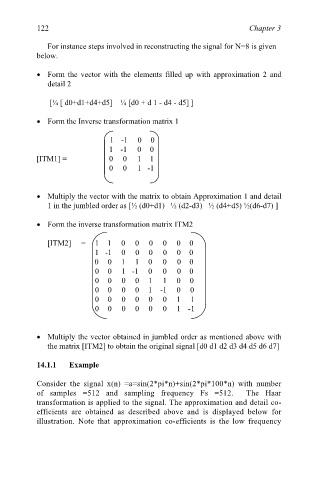
For instance steps involved in reconstructing the signal for N=8 is given
below.

• Form the vector with the elements filled up with approximation 2 and
detail 2

[¼ [ d0+d1+d4+d5] ¼ [d0 + d 1 - d4 - d5] ]

• Form the Inverse transformation matrix 1

1 -1 0 0

1 -1 0 0
[ITM1] = 0 0 1 1
0 0 1 -1

• Multiply the vector with the matrix to obtain Approximation 1 and detail
1 in the jumbled order as [½ (d0+d1) ½ (d2-d3) ½ (d4+d5) ½(d6-d7) ]

• Form the inverse transformation matrix ITM2

[ITM2] = 1 1 0 0 0 0 0 0

1 -1 0 0 0 0 0 0
0 0 1 1 0 0 0 0
0 0 1 -1 0 0 0 0
0 0 0 0 1 1 0 0
0 0 0 0 1 -1 0 0
0 0 0 0 0 0 1 1
0 0 0 0 0 0 1 1
-

• Multiply the vector obtained in jumbled order as mentioned above with
the matrix [ITM2] to obtain the original signal [d0 d1 d2 d3 d4 d5 d6 d7]

14.1.1 Example

Consider the signal x(n) =a=sin(2*pi*n)+sin(2*pi*100*n) with number
of samples =512 and sampling frequency Fs =512. The Haar
transformation is applied to the signal. The approximation and detail co-
efficients are obtained as described above and is displayed below for
illustration. Note that approximation co-efficients is the low frequency