Page 73 - Algorithm Collections for Digital Signal Processing Applications using MATLAB

2. Probability and Random Process 61

T
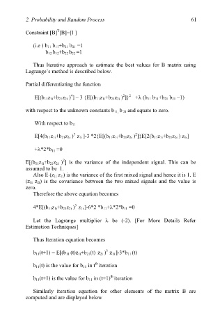
Constraint [B] [B]=[I ]
(i.e ) b 11 b 11+b 21 b 21 =1
b 12 b 12+b 22 b 22 =1

Thus Iterative approach to estimate the best values for B matrix using
Lagrange’s method is described below.

Partial differentiating the function

4
2
E[(b 11z 1i+b 21z 2i ) ] – 3 {E[(b 11z 1i+b 21z 2i ) ]} 2 +λ (b 11 b 11+b 21 b 21 –1)
with respect to the unknown constants b 11, b 21 and equate to zero.

With respect to b 11

3
2
E[4(b 11z 1i+b 21z 2i ) z 1i ]-3 *2{E[(b 11z 1i+b 21z 2i ) ]}E[2(b 11z 1i+b 21z 2i ) z 1i]
+λ*2*b 11 =0

2
E[(b 11z 1i+b 21z 2i ) ] is the variance of the independent signal. This can be
assumed to be 1.
Also E (z 1i z 1i) is the variance of the first mixed signal and hence it is 1. E
(z 1i z 2i) is the covariance between the two mixed signals and the value is
zero.
Therefore the above equation becomes

3
4*E[(b 11z 1i+b 21z 2i ) z 1i ]-6*2 *b 11+λ*2*b 11 =0
Let the Lagrange multiplier λ be (-2). [For More Details Refer
Estimation Techniques]

Thus Iteration equation becomes

3
b 11(t+1) = E[(b 11 (t)z 1i+b 21(t) z 2i ) z 1i ]-3*b 11 (t)
th
b 11(t) is the value for b 11 in t iteration
th
b 11(t+1) is the value for b 11 in (t+1) iteration

Similarly iteration equation for other elements of the matrix B are
computed and are displayed below