Page 69 - Algorithm Collections for Digital Signal Processing Applications using MATLAB

2. Probability and Random Process 57

To compare the covariance matrix, correlation coefficient is used. It is the
normalized covariance matrix whose (m, n) element is computed as
COV( m, n) / (sqrt(COV(m,m)*COV(n,n))
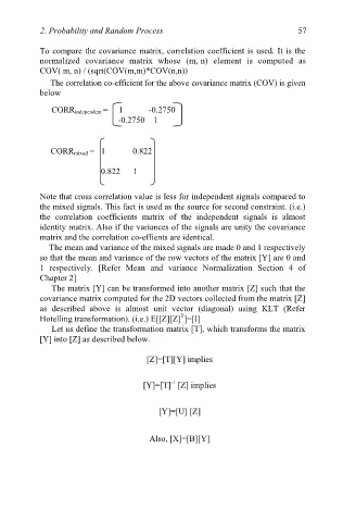
The correlation co-efficient for the above covariance matrix (COV) is given
below

CORR independent = 1 -0.2750
-0.2750 1

CORR mixed = 1 0.822

0.822 1

Note that cross correlation value is less for independent signals compared to
the mixed signals. This fact is used as the source for second constraint. (i.e.)
the correlation coefficients matrix of the independent signals is almost
identity matrix. Also if the variances of the signals are unity the covariance
matrix and the correlation co-effients are identical.
The mean and variance of the mixed signals are made 0 and 1 respectively
so that the mean and variance of the row vectors of the matrix [Y] are 0 and
1 respectively. [Refer Mean and variance Normalization Section 4 of
Chapter 2]
The matrix [Y] can be transformed into another matrix [Z] such that the
covariance matrix computed for the 2D vectors collected from the matrix [Z]
as described above is almost unit vector (diagonal) using KLT (Refer
T
Hotelling transformation). (i.e.) E[[Z][Z] ]=[I]
Let us define the transformation matrix [T], which transforms the matrix
[Y] into [Z] as described below.

[Z]=[T][Y] implies

-1
[Y]=[T] [Z] implies

[Y]=[U] [Z]

Also, [X]=[B][Y]