
Page 282 -
P. 282
256 Chapter 7 ■ Image Restoration
work fine, but is very slow, and it would not likely be used in any real system.
Because of the very useful nature of the Fourier transform, an enormous
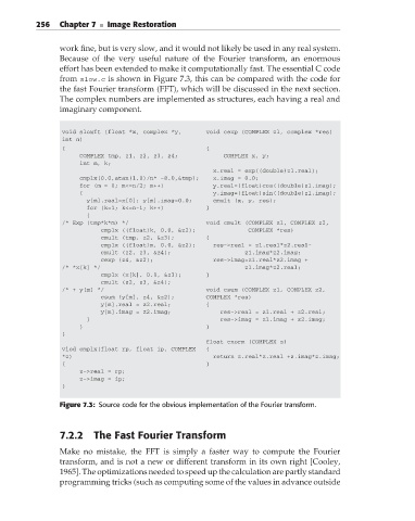
effort has been extended to make it computationally fast. The essential C code
from slow.c is shown in Figure 7.3, this can be compared with the code for
the fast Fourier transform (FFT), which will be discussed in the next section.
The complex numbers are implemented as structures, each having a real and
imaginary component.
void slowft (float *x, complex *y, void cexp (COMPLEX zl, complex *res)
int n)
{ {
COMPLEX tmp, z1, z2, z3, z4; COMPLEX x, y;
int m, k;
x.real = exp((double)zl.real);
cmplx(0.0,atan(1.0)/n* -8.0,&tmp); x.imag = 0.0;
for (m = 0; m<=n/2; m++) y.real=(float)cos((double)zl.imag);
{ y.imag=(float)sin((double)zl.imag);
y[m].real=x[0]; y[m].imag=0.0; cmult (x, y, res);
for (k=1; k<=n-1; k++) }
{
/* Exp (tmp*k*m) */ void cmult (COMPLEX zl, COMPLEX z2,
cmplx ((float)k, 0.0, &z2); COMPLEX *res)
cmult (tmp, z2, &z3); {
cmplx ((float)m, 0.0, &z2); res->real = z1.real*z2.real-
cmult (z2, z3, &z4); z1.imag*z2.imag;
cexp (z4, &z2); res->imag=z1.real*z2.imag +
/* *x[k] */ z1.imag*z2.real;
cmplx (x[k], 0.0, &z3); }
cmult (z2, z3, &z4);
/* + y[m] */ void csum (COMPLEX z1, COMPLEX z2,
csum (y[m], z4, &z2); COMPLEX *res)
y[m].real = z2.real; {
y[m].imag = z2.imag; res->real = z1.real + z2.real;
} res->imag = z1.imag + z2.imag;
} }
}
float cnorm (COMPLEX z)
viod cmplx(float rp, float ip, COMPLEX {
*z) return z.real*z.real +z.imag*z.imag;
{ }
z->real = rp;
z->imag = ip;
}
Figure 7.3: Source code for the obvious implementation of the Fourier transform.
7.2.2 The Fast Fourier Transform
Make no mistake, the FFT is simply a faster way to compute the Fourier
transform, and is not a new or different transform in its own right [Cooley,
1965]. The optimizations needed to speed up the calculation are partly standard
programming tricks (such as computing some of the values in advance outside