
Page 283 -
P. 283
Chapter 7 ■ Image Restoration 257
of the loop) and partly mathematical techniques. There are a number of
very good references on the FFT [Bracewell, 1965; Brigham, 1974], but these
deal rather rigorously with the subject. Here, the code in Figure 7.3 will be
successively improved until it implements the basic FFT method.
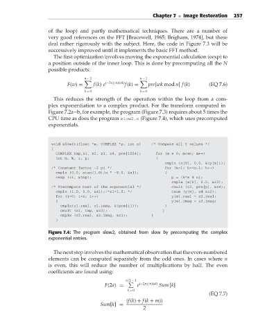
The first optimization involves moving the exponential calculation (cexp) to
a position outside of the inner loop. This is done by precomputing all the N
possible products:
n − 1 n − 1
(−2πj/n)(wk)
F(w) = f(k) e f(k) = pre[wk mod n] f(k) (EQ 7.6)
k = 0 k = 0
This reduces the strength of the operation within the loop from a com-
plex exponentiation to a complex product. For the transform computed in
Figure 7.2a–b, for example, the program (Figure 7.3) requires about 5 times the
CPU time as does the program slow2.c (Figure 7.4), which uses precomputed
exponentials.
void slowft(float *x, COMPLEX *y, int n) /* Compute all Y values */
{
COMPLEX tmp,z1, z2, z3, z4, pre[1024]; for (m = 0; m<=n; m++)
int m, k, i, p; {
cmplx (x[0], 0.0, &(y[m]));
/* Constant factor -2 pi */ for (k=1; k<=n-1; k++)
cmplx (0.0, atan(1.0)/n * -8.0, &z1); {
cexp (z1, &tmp); p = (k*m % n);
cmplx (x[k], 0.0, &z3);
/* Precompute most of the exponential */ cmult (z3, pre[p], &z4);
cmplx (1.0, 0.0, &z1);/*z1=1.0; */ csum (y[m], z4 &z2);
for (i=0; i<n; i++) y[m].real = z2.real;
{ y[m].imag = z2.imag;
cmplx(z1.real, z1.imag, &(pre[i])); }
cmult (z1, tmp, &z3); }
cmplx (z3.real, z3.imag, &z1); }
}
Figure 7.4: The program slow2, obtained from slow by precomputing the complex
exponential entries.
The next step involves the mathematical observation that the even-numbered
elements can be computed separately from the odd ones. In cases where n
is even, this will reduce the number of multiplications by half. The even
coefficients are found using:
n/2 − 1
(−2πj/n)(ak)
F(2a) = e Sum [k]
k = 0
(EQ 7.7)
(f(k) + f(k + m))
Sum[k] =
2