Page 53 -

Chapter 2 ■ Edge-Detection Techniques 27

the standard deviation of the grey levels will be close to that of the noise. To
make sure that this is working properly, we can now use the mean already
computed as the grey level of the square and compute the mean and standard
deviation of the difference of each grey level from the mean;thisnew mean should
be near to zero, and the standard deviation close to that of that noise (and to
the previously computed standard deviation).

(a) (b) (c)

(d) (e) (f)
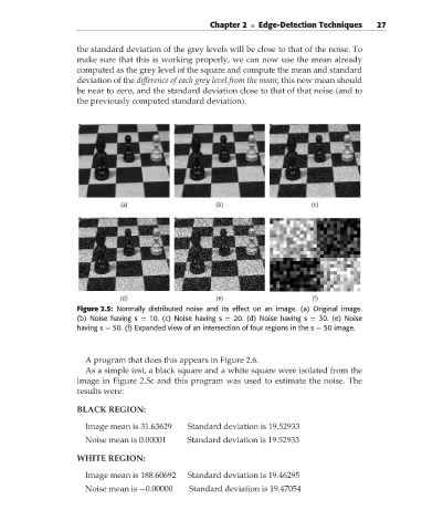
Figure 2.5: Normally distributed noise and its effect on an image. (a) Original image.
(b) Noise having s = 10. (c) Noise having s = 20. (d) Noise having s = 30. (e) Noise
having s = 50. (f) Expanded view of an intersection of four regions in the s = 50 image.

A program that does this appears in Figure 2.6.
As a simple test, a black square and a white square were isolated from the
image in Figure 2.5c and this program was used to estimate the noise. The
results were:

BLACK REGION:

Image mean is 31.63629 Standard deviation is 19.52933
Noise mean is 0.00001 Standard deviation is 19.52933

WHITE REGION:

Image mean is 188.60692 Standard deviation is 19.46295
Noise mean is −0.00000 Standard deviation is 19.47054