Page 75 -

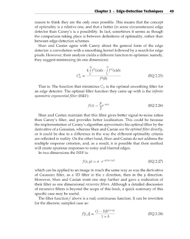
Chapter 2 ■ Edge-Detection Techniques 49

reason to think they are the only ones possible. This means that the concept
of optimality is a relative one, and that a better (in some circumstances) edge
detector than Canny’s is a possibility. In fact, sometimes it seems as though
the comparison taking place is between definitions of optimality, rather than
between edge-detection schemes.
Shen and Castan agree with Canny about the general form of the edge
detector: a convolution with a smoothing kernel followed by a search for edge
pixels. However, their analysis yields a different function to optimize: namely,
they suggest minimizing (in one dimension):

∞ ∞

2 2
4 f (x)dx · f (x)dx
2 0 0
C = (EQ 2.25)
N
4
f (0)
That is: The function that minimizes C N is the optimal smoothing filter for
an edge detector. The optimal filter function they came up with is the infinite
symmetric exponential filter (ISEF):
p
f(x) = e −p|x| (EQ 2.26)
2
Shen and Castan maintain that this filter gives better signal-to-noise ratios
than Canny’s filter, and provides better localization. This could be because
the implementation of Canny’s algorithm approximates his optimal filter by the
derivative of a Gaussian, whereas Shen and Castan use the optimal filter directly,
or it could be due to a difference in the way the different optimality criteria
are reflected in reality. On the other hand, Shen and Castan do not address the
multiple response criterion, and, as a result, it is possible that their method
will create spurious responses to noisy and blurred edges.
In two dimensions the ISEF is:

f(x, y) = a · e −p(|x|+|y|) (EQ 2.27)

which can be applied to an image in much the same way as was the derivative
of Gaussian filter, as a 1D filter in the x direction, then in the y direction.
However, Shen and Castan went one step further and gave a realization of
their filter as one dimensional recursive filters. Although a detailed discussion
of recursive filters is beyond the scope of this book, a quick summary of this
specific case may be useful.
The filter function f above is a real, continuous function. It can be rewritten
for the discrete, sampled case as:

(1 − b)b |x|+|y|
f[i, j] = (EQ 2.28)
1 + b