Page 73 -

Chapter 2 ■ Edge-Detection Techniques 47

point, which is at location (P x , P y ). In Figure 2.13 the crossing point is marked
with a ‘‘+’’, and is in between B and C. The gradient magnitude at this point
is estimated as
G = (P y − C y )Norm(C) + (B y − P y )Norm(B) (EQ 2.24)

where the norm function computes the gradient magnitude.
Every pixel in the filtered image is processed in this way; the gradient
magnitude is estimated for two locations, one on each side of the pixel, and the
magnitude at the pixel must be greater than its neighbors’. In the general case
there are eight major cases to check for, and some short cuts that can be made
for efficiency’s sake, but the above method is essentially what is used in most
implementations of the Canny edge detector. The function nonmax_suppress
in the C source at the end of the chapter computes a value for the magnitude
at each pixel based on this method, and sets the value to zero unless the pixel
is a local maximum.
It would be possible to stop at this point and use the method to enhance
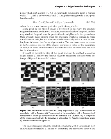
edges. Figure 2.14 shows the various stages in processing the chessboard test
image of Figure 2.8 (no added noise).

(a) (b) (c)

(d) (e) (f)
Figure 2.14: Intermediate results from the Canny edge detector. (a) X component of the
convolution with a Gaussian. (b) Y component of the convolution with a Gaussian. (c) X
component of the image convolved with the derivative of a Gaussian. (d) Y component
of the image convolved with the derivative of a Gaussian. (e) Resulting magnitude image.
(f) After non-maximum suppression.

The stages are: computing the result of convolving with a Gaussian in the x
and y directions (Figures 2.14a and b); computing the derivatives in the x and