Page 626 -

606 CHAPTER 14 MULTICRITERIA DECISIONS

To solve the Suncoast Office Supplies problem, we begin by solving the P 1 problem:
þ
Min d þ d
2
1
s:t:
þ
2E þ 3N d þ d ¼ 680 Goal 1
1 1
þ
2E þ 3N d þ d ¼ 600 Goal 2
2
2
þ
250E þ 125N d þ d ¼ 70 000 Goal 3
3 3
þ
E d þ d ¼ 200 Goal 4
4
4
þ
N d þ d ¼ 120 Goal 5
5 5
þ

þ

þ

þ

þ
E; N; d ; d ; d ; d ; d ; d ; d ; d ; d ; d 0
2
2
1
1
3
5
5
4
3
4
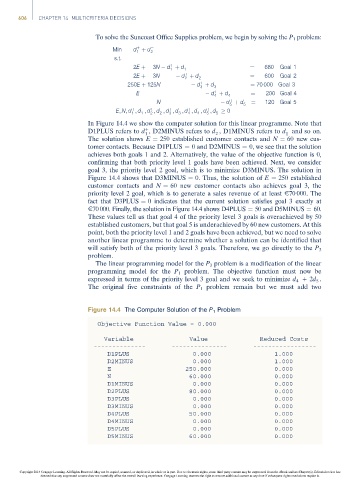
In Figure 14.4 we show the computer solution for this linear programme. Note that

þ

D1PLUS refers to d , D2MINUS refers to d , D1MINUS refers to d and so on.
1 2 1
The solution shows E ¼ 250 established customer contacts and N ¼ 60 new cus-
tomer contacts. Because D1PLUS ¼ 0 and D2MINUS ¼ 0, we see that the solution
achieves both goals 1 and 2. Alternatively, the value of the objective function is 0,
confirming that both priority level 1 goals have been achieved. Next, we consider
goal 3, the priority level 2 goal, which is to minimize D3MINUS. The solution in
Figure 14.4 shows that D3MINUS ¼ 0. Thus, the solution of E ¼ 250 established
customer contacts and N ¼ 60 new customer contacts also achieves goal 3, the
priority level 2 goal, which is to generate a sales revenue of at least E70 000. The
fact that D3PLUS ¼ 0 indicates that the current solution satisfies goal 3 exactly at
E70000. Finally, the solution in Figure 14.4 shows D4PLUS ¼ 50 and D5MINUS ¼ 60.
These values tell us that goal 4 of the priority level 3 goals is overachieved by 50
established customers, but that goal 5 is underachieved by 60 new customers. At this
point, both the priority level 1 and 2 goals have been achieved, but we need to solve
another linear programme to determine whether a solution can be identified that
will satisfy both of the priority level 3 goals. Therefore, we go directly to the P 3
problem.
The linear programming model for the P 3 problem is a modification of the linear
programming model for the P 1 problem. The objective function must now be

expressed in terms of the priority level 3 goal and we seek to minimize d 4 +2d 5 .
The original five constraints of the P 1 problem remain but we must add two
Figure 14.4 The Computer Solution of the P 1 Problem
Objective Function Value = 0.000
Variable Value Reduced Costs
-------------- --------------- -----------------
D1PLUS 0.000 1.000
D2MINUS 0.000 1.000
E 250.000 0.000
N 60.000 0.000
D1MINUS 0.000 0.000
D2PLUS 80.000 0.000
D3PLUS 0.000 0.000
D3MINUS 0.000 0.000
D4PLUS 50.000 0.000
D4MINUS 0.000 0.000
D5PLUS 0.000 0.000
D5MINUS 60.000 0.000
Copyright 2014 Cengage Learning. All Rights Reserved. May not be copied, scanned, or duplicated, in whole or in part. Due to electronic rights, some third party content may be suppressed from the eBook and/or eChapter(s). Editorial review has
deemed that any suppressed content does not materially affect the overall learning experience. Cengage Learning reserves the right to remove additional content at any time if subsequent rights restrictions require it.