Page 265 - Analysis, Synthesis and Design of Chemical Processes, Third Edition

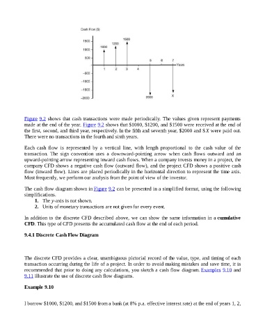
Figure 9.2 shows that cash transactions were made periodically. The values given represent payments

made at the end of the year. Figure 9.2 shows that $1000, $1200, and $1500 were received at the end of
the first, second, and third year, respectively. In the fifth and seventh year, $2000 and $ X were paid out.
There were no transactions in the fourth and sixth years.

Each cash flow is represented by a vertical line, with length proportional to the cash value of the
transaction. The sign convention uses a downward-pointing arrow when cash flows outward and an
upward-pointing arrow representing inward cash flows. When a company invests money in a project, the
company CFD shows a negative cash flow (outward flow), and the project CFD shows a positive cash
flow (inward flow). Lines are placed periodically in the horizontal direction to represent the time axis.
Most frequently, we perform our analysis from the point of view of the investor.

The cash flow diagram shown in Figure 9.2 can be presented in a simplified format, using the following
simplifications.
1. The y-axis is not shown.
2. Units of monetary transactions are not given for every event.

In addition to the discrete CFD described above, we can show the same information in a cumulative
CFD. This type of CFD presents the accumulated cash flow at the end of each period.

9.4.1 Discrete Cash Flow Diagram

The discrete CFD provides a clear, unambiguous pictorial record of the value, type, and timing of each
transaction occurring during the life of a project. In order to avoid making mistakes and save time, it is
recommended that prior to doing any calculations, you sketch a cash flow diagram. Examples 9.10 and
9.11 illustrate the use of discrete cash flow diagrams.

Example 9.10

I borrow $1000, $1200, and $1500 from a bank (at 8% p.a. effective interest rate) at the end of years 1, 2,