Page 270 - Analysis, Synthesis and Design of Chemical Processes, Third Edition

X = $3057.99 ≈ $3058
b. For i = 0.00
Withdrawals = $1000 + $1200 + $1500 = $3700
Repayments = – $(2000 + X)
0 = $3700 – $(2000 + X)
X = $1700

Note: Because of the interest paid to the bank, the borrower repaid a total of $1358 ($3058 – $1700)
more than was borrowed from the bank seven years earlier.

To demonstrate that any point in time could be used, as a basis, compare the amount repaid based on the
end of year 1. Equation (9.6) is used, and all cash flows are moved backward in time (exponents become
negative). This gives

and solving for X yields

= $3058 (the same answer as before!)

Usually, the desire is to compute investments at the start or at the end of a project, but the conclusions
drawn are independent of where that comparison is made.

9.5.1 Annuities—A Uniform Series of Cash Transactions

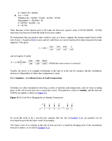
Problems are often encountered involving a series of uniform cash transactions, each of value A, taking
place at the end of each year for n consecutive years. This pattern is called an annuity, and the discrete
CFD for an annuity is shown in Figure 9.3.

Figure 9.3 A Cash Flow Diagram for an Annuity Transaction

To avoid the need to do a year-by-year analysis like the one in Example 9.13, an equation can be
developed to provide the future value of an annuity.

The future value of an annuity at the end of time period n is found by bringing each of the investments
forward to time n, as we did in Example 9.13.