Page 59 - Anatomy of a Robot

02_200256_CH02/Bergren 4/17/03 11:23 AM Page 44
44 CHAPTER TWO
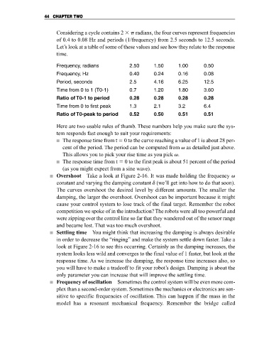
Considering a cycle contains 2 p radians, the four curves represent frequencies
of 0.4 to 0.08 Hz and periods (1/frequency) from 2.5 seconds to 12.5 seconds.
Let’s look at a table of some of these values and see how they relate to the response
time.
Frequency, radians 2.50 1.50 1.00 0.50
Frequency, Hz 0.40 0.24 0.16 0.08
Period, seconds 2.5 4.16 6.25 12.5
Time from 0 to 1 (T0-1) 0.7 1.20 1.80 3.60
Ratio of T0-1 to period 0.28 0.28 0.28 0.28
Time from 0 to first peak 1.3 2.1 3.2 6.4
Ratio of T0-peak to period 0.52 0.50 0.51 0.51
Here are two usable rules of thumb. These numbers help you make sure the sys-
tem responds fast enough to suit your requirements:
The response time from t 0 to the curve reaching a value of 1 is about 28 per-
cent of the period. The period can be computed from v as detailed just above.
This allows you to pick your rise time as you pick v.
The response time from t 0 to the first peak is about 51 percent of the period
(as you might expect from a sine wave).
Overshoot Take a look at Figure 2-16. It was made holding the frequency v
constant and varying the damping constant d (we’ll get into how to do that soon).
The curves overshoot the desired level by different amounts. The smaller the
damping, the larger the overshoot. Overshoot can be important because it might
cause your control system to lose track of the final target. Remember the robot
competition we spoke of in the introduction? The robots were all too powerful and
were zipping over the control line so far that they wandered out of the sensor range
and became lost. That was too much overshoot.
Settling time You might think that increasing the damping is always desirable
in order to decrease the “ringing” and make the system settle down faster. Take a
look at Figure 2-16 to see this occurring. Certainly as the damping increases, the
system looks less wild and converges to the final value of 1 faster, but look at the
response time. As we increase the damping, the response time increases also, so
you will have to make a tradeoff to fit your robot’s design. Damping is about the
only parameter you can increase that will improve the settling time.
Frequency of oscillation Sometimes the control system will be even more com-
plex than a second-order system. Sometimes the mechanics or electronics are sen-
sitive to specific frequencies of oscillation. This can happen if the mass in the
model has a resonant mechanical frequency. Remember the bridge called