Page 200 - Applied Numerical Methods Using MATLAB

SECANT METHOD 189
20
2
1 10
x 0
0 x 0 x 3
x 1 x 2 x 3
0
−1 x 2 x 1
−2 −10
1.8 2 2.2 2.4 2.6 0 5 10 15 20
1 2
(a) f 42 (x) = tan (p − x) − x (b) f 44b (x) = (x − 25)(x − 10) − 5
125
2
x 0 x 1 x 2 x 3
0
1
−10
x 2 x 1
−20 0 x 0
x 3
−30
−1
−40
−2
−15 −10 −5 0 5 10 15 −5 0 5 10
1 2 −1
(c) f 44b (x) = (x − 25)(x − 10) − 5 (d) f 44d (x) = tan (x − 2)
125
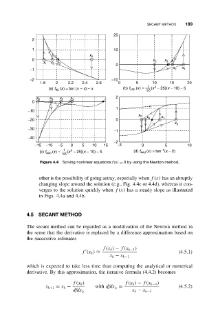
Figure 4.4 Solving nonlinear equations f(x) = 0 by using the Newton method.

other is the possibility of going astray, especially when f(x) has an abruptly
changing slope around the solution (e.g., Fig. 4.4c or 4.4d), whereas it con-
verges to the solution quickly when f(x) has a steady slope as illustrated
in Figs. 4.4a and 4.4b.

4.5 SECANT METHOD
The secant method can be regarded as a modification of the Newton method in
the sense that the derivative is replaced by a difference approximation based on
the successive estimates
f(x k ) − f(x k−1 )

f (x k ) ≈ (4.5.1)
x k − x k−1
which is expected to take less time than computing the analytical or numerical
derivative. By this approximation, the iterative formula (4.4.2) becomes

f(x k ) f(x k ) − f(x k−1 )
x k+1 = x k − with dfdx = (4.5.2)
k
dfdx k x k − x k−1