Page 204 - Applied Numerical Methods Using MATLAB

SYMBOLIC SOLUTION FOR EQUATIONS 193
2
2x 1 − 2x 1 − 3x 2 = 2.5
1 1 1
1 0
0
0 0
−1 2 2 −1
x 1 + 4x 2 = 5
−3 −2 −1 0 1 2 3 −3 −2 −1 0 1 2 3
(a) Newton method with (x 10 , x 20 ) = (0.8, 0.2) (b) Newton method with (x 10 , x 20 ) = (−1.0, 0.5)
4
2
2
0 0
0 1
6 5 4 3 2 1
−2
−4
−5 0 5 −3 −2 −1 0 1 2 3
(c) Newton method with (x 10 , x 20 ) = (0.5, 0.2) (d) Damped Newton method with
(x 10 , x 20 ) = (0.5, 0.2)
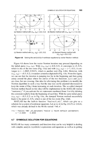
Figure 4.6 Solving the set (4.6.6) of nonlinear equations by vector Newton method.

Figure 4.6 shows how the vector Newton iteration may proceed depending on
the initial guess (x 10 ,x 20 ). With (x 10 ,x 20 ) = (0.8, 0.2), it converges to (2, 0.5),
which is one of the two roots (Fig. 4.6a) and with (x 10 ,x 20 ) = (−1, 0.5), it con-
verges to (−1.2065, 0.9413), which is another root (Fig. 4.6b). However, with
(x 10 ,x 20 ) = (0.5, 0.2), it wanders around as depicted in Fig. 4.6c. From this figure,
we can see that the iteration is jumping too far in the beginning and then going
astray around the place where the curves of the two functions f 1 (x) and f 2 (x)
are close, but not crossing. One idea for alleviating this problem is to modify the
Newton algorithm in such a way that the step size can be adjusted (decreased) to
keep the norm of f(x k ) from increasing at each iteration. The so-called damped
Newton method based on this idea will be implemented in the MATLAB routine
“newtons()” if you activate the six statements numbered from 1 to 6 by deleting
the comment mark(%) from the beginning of each line. With the same initial guess
(x 10 ,x 20 ) = (0.5, 0.2) as in Fig. 4.6c, the damped Newton method successfully
leads to the point (2, 0.5), which is one of the two roots (Fig. 4.6d).
MATLAB has the built-in function “fsolve(f,x0)”, which can give us a
solution for a system of nonlinear equations. Let us try it for Eq. (4.6.5) or (4.6.6),
which was already defined in the M-file named ‘f46.m’.

>>x = fsolve(’f46’,x0,optimset(’fsolve’)) %with default parameters
x = 2.0000 0.5000

4.7 SYMBOLIC SOLUTION FOR EQUATIONS

MATLAB has many commands and functions that can be very helpful in dealing
with complex analytic (symbolic) expressions and equations as well as in getting