Page 209 - Applied Numerical Methods Using MATLAB

198 NONLINEAR EQUATIONS

6 3
1
2
y = g a (x) = (x + 1) y = g b (x) = 3 − 1 x o2
3 x
5 2.5
4 2

3 o2 1.5
x
y = x y = x
2 1

1 0.5 x o1
x o1
0 0

−1 −0.5
0 2 4 6 0 1 2 3
1
2
(a) x k + 1 = g a (x k ) = (x k + 1) (b) x k + 1 = g b (x k ) = 3 − 1
3 x k
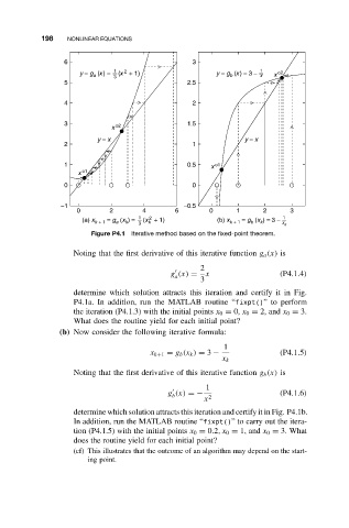
Figure P4.1 Iterative method based on the fixed-point theorem.
Noting that the first derivative of this iterative function g a (x) is

2

g (x) = x (P4.1.4)
a
3
determine which solution attracts this iteration and certify it in Fig.
P4.1a. In addition, run the MATLAB routine “fixpt()” to perform
the iteration (P4.1.3) with the initial points x 0 = 0, x 0 = 2, and x 0 = 3.
What does the routine yield for each initial point?
(b) Now consider the following iterative formula:
1
x k+1 = g b (x k ) = 3 − (P4.1.5)
x k
Noting that the first derivative of this iterative function g b (x) is

1

g (x) =− (P4.1.6)
b 2
x
determine which solution attracts this iteration and certify it in Fig. P4.1b.
In addition, run the MATLAB routine “fixpt()” to carry out the itera-
tion (P4.1.5) with the initial points x 0 = 0.2,x 0 = 1, and x 0 = 3. What
does the routine yield for each initial point?
(cf) This illustrates that the outcome of an algorithm may depend on the start-
ing point.