Page 213 - Applied Numerical Methods Using MATLAB

202 NONLINEAR EQUATIONS
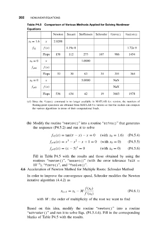
Table P4.5 Comparison of Various Methods Applied for Solving Nonlinear
Equations
Newton Secant Steffensen Schroder fzero() fsolve()

x 0 = 1.6 x 2.0288
f 42 f(x) 1.19e-8 1.72e-9
Flops 158 112 273 167 986 1454

x 0 = 0 x 1.0000
f p44 f(x)
Flops 53 30 63 31 391 364
x 0 = 0 x 5.0000 NaN

f(x) NaN
f p45
Flops 536 434 42 19 3683 1978

(cf) Since the flops() command is no longer available in MATLAB 6.x version, the numbers of
floating-point operations are obtained from MATLAB 5.x version so that the readers can compare
the various algorithms in terms of their computational loads.

(b) Modify the routine “newton()” into a routine “stfns()” that generates
the sequence (P4.5.2) and run it to solve
f 42 (x) = tan(π − x) − x = 0 (with x 0 = 1.6) (P4.5.4)
3 2
f p44 (x) = x − x − x + 1 = 0 (with x 0 = 0) (P4.5.5)
4
f p45 (x) = (x − 5) = 0 (with x 0 = 0) (P4.5.6)

Fill in Table P4.5 with the results and those obtained by using the
routines “newton()”, “secant()” (with the error tolerance TolX =
−5
10 ), “fzero()”, and “fsolve()”.
4.6 Acceleration of Newton Method for Multiple Roots: Schroder Method
In order to improve the convergence speed, Schroder modifies the Newton
iterative algorithm (4.4.2) as

f(x k )
x k+1 = x k − M (P4.6.1)
f (x k )

with M : the order of multiplicity of the root we want to find

Based on this idea, modify the routine “newton()” into a routine
“schroder()” and run it to solve Eqs. (P4.5.4.6). Fill in the corresponding
blanks of Table P4.5 with the results.