Page 208 - Applied Numerical Methods Using MATLAB

PROBLEMS 197

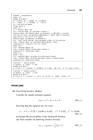
%nm4e03 – astrophysics
clear, clf
global G Ms Me R T
G = 6.67e11; Ms = 1.98e30; Me = 5.98e24;
R = 1.49e11; T = 3.15576e7; w = 2*pi/T;
x0 = 1e6 %initial guess
format short e
disp(’(a)’)
rn = newtons(’phys’,x0)
rfs = fsolve(’phys’,x0 ,optimset(’fsolve’))
%fsolve(’phys’,x0)/fsolve(’phys’,x0,foptions) in MATLAB 5.x version
rfs1=fsolve(’phys’,x0,optimset(’MaxFunEvals’,1000)) %more iterations
%options([2 3 14])=[1e-4 1e-4 1000];
%fsolve(’phys’,x0,options) in MATLAB 5.x
x01 = 1e10; %with another starting guess closer to the solution
rfs2 = fsolve(’phys’,x01,optimset(’MaxFunEvals’,1000))
residual_errs = phys([rn rfs rfs1 rfs2])
disp(’(b)’)
rnb = newtons(’physb’,x0)
rfsb = fsolve(’physb’,x0,optimset(’fsolve’))
residual_errs = phys([rnb rfsb])
disp(’(c)’)
scale = 1e11;
rns = newtons(’phys’,x0/scale,1e-6,100,scale)*scale;
rfss = fsolve(’phys’,x0/scale,optimset(’fsolve’),scale)*scale
residual_errs = phys([rns rfss])
function f = phys(x,scale);
if nargin < 2, scale = 1; end
global G Ms Me R T
w = 2*pi/T; x = x*scale; f = G*(Ms/(x.^2 + eps) - Me./((R - x).^2 + eps))-x*w^2;
function f = physb(x,scale);
if nargin < 2, scale = 1; end
global G Ms Me R T
w = 2*pi/T; x = x*scale; f = (R-x).^2.*(w^2*x.^3 - G*Ms) + G*Me*x.^2;

PROBLEMS

4.1 Fixed-Point Iterative Method
Consider the simple nonlinear equation

2
f(x) = x − 3x + 1 = 0 (P4.1.1)
Knowing that this equation has two roots

√
o o1 o2
x = 1.5 ± 1.25 ≈ 2.6180 or 0.382; x ≈ 0.382,x ≈ 2.6180
(P4.1.2)
investigate the practicability of the fixed-point iteration.
(a) First consider the following iterative formula:

1 2
x k+1 = g a (x k ) = (x + 1) (P4.1.3)
k
3