Page 207 - Applied Numerical Methods Using MATLAB

196 NONLINEAR EQUATIONS
(b) Noting that Eq. (E4.3.1) may cause ‘division-by-zero’, we multiply both
2
2
sides of the equation by r (R − r) to rewrite it as
3
2
2
2
2
r (R − r) ω − GM S (R − r) + GM e r = 0 (E4.3.2)
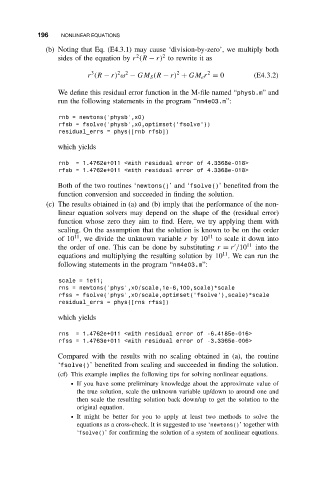
We define this residual error function in the M-file named “physb.m”and
run the following statements in the program “nm4e03.m”:
rnb = newtons(’physb’,x0)
rfsb = fsolve(’physb’,x0,optimset(’fsolve’))
residual_errs = phys([rnb rfsb])

which yields

rnb = 1.4762e+011 <with residual error of 4.3368e-018>
rfsb = 1.4762e+011 <with residual error of 4.3368e-018>

Both of the two routines ‘newtons()’and ‘fsolve()’ benefited from the
function conversion and succeeded in finding the solution.
(c) The results obtained in (a) and (b) imply that the performance of the non-
linear equation solvers may depend on the shape of the (residual error)
function whose zero they aim to find. Here, we try applying them with
scaling. On the assumption that the solution is known to be on the order
11
of 10 , we divide the unknown variable r by 10 11 to scale it down into
the order of one. This can be done by substituting r = r /10 11 into the

11
equations and multiplying the resulting solution by 10 . We can run the
following statements in the program “nm4e03.m”:
scale = 1e11;
rns = newtons(’phys’,x0/scale,1e-6,100,scale)*scale
rfss = fsolve(’phys’,x0/scale,optimset(’fsolve’),scale)*scale
residual_errs = phys([rns rfss])

which yields

rns = 1.4762e+011 <with residual error of -6.4185e-016>
rfss = 1.4763e+011 <with residual error of -3.3365e-006>
Compared with the results with no scaling obtained in (a), the routine
‘fsolve()’ benefited from scaling and succeeded in finding the solution.
(cf) This example implies the following tips for solving nonlinear equations.
ž If you have some preliminary knowledge about the approximate value of
the true solution, scale the unknown variable up/down to around one and
then scale the resulting solution back down/up to get the solution to the
original equation.
ž It might be better for you to apply at least two methods to solve the
equations as a cross-check. It is suggested to use ‘newtons()’ together with
‘fsolve()’ for confirming the solution of a system of nonlinear equations.