Page 206 - Applied Numerical Methods Using MATLAB

A REAL-WORLD PROBLEM 195

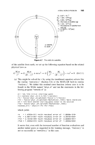
E G = 6.67 × 10 −11
30
s M s = 1.98 × 10 [kg]
24
M e = 5.98 × 10 [kg]
m = the mass of satellite [kg]
11
R = 1.49 × 10 [m]
g = the distance of satellite from
sun [m]
7
T = 3.15576 × 10 [sec]
w = 2p/T
E s Sun s E

s: satellite
g E: earth
R

s
E
Figure 4.7 The orbit of a satellite.

of the satellite from earth, we set up the following equation based on the related
physical laws as

M s m M e m 2 M S M e 2
G = G + mrω → G − − rω = 0 (E4.3.1)
r 2 (R − r) 2 r 2 (R − r) 2
(a) This might be solved for r by using the (nonlinear) equation solvers like
the routine ‘newtons()’ (Section 4.6) or the MATLAB built-in routine
‘fsolve()’. We define this residual error function (whose zero is to be
found) in the M-file named “phys.m” and run the statements in the fol-
lowing program “nm4e03.m”as

x0 = 1e6; %the initial (starting) guess
rn = newtons(’phys’,x0,1e-4,100) % newtons()
rfs = fsolve(’phys’,x0,optimset(’fsolve’)) % fsolve()
rfs1 = fsolve(’phys’,x0,optimset(’MaxFunEvals’,1000)) %more iterations
x01 = 1e10 %with another starting guess closer to the solution
rfs2 = fsolve(’phys’,x01,optimset(’MaxFunEvals’,1000))
residual_errs = phys([rn rfs rfs1 rfs2])

which yields
rn = 1.4762e+011 <with residual error of -1.8908e-016>
rfs = 5.6811e+007 <with residual error of 4.0919e+004>
rfs1 = 2.1610e+009 <with residual error of 2.8280e+001>
rfs2 = 1.0000e+010 <with residual error of 1.3203e+000>

It seems that, even with the increased number of function evaluations and
another initial guess as suggested in the warning message, ‘fsolve()’is
not so successful as ‘newtons()’ in this case.