Page 334 - Applied Numerical Methods Using MATLAB

UNCONSTRAINED OPTIMIZATION 323

2

a 3 c 3 d 3 b 3
1 a 2 c 2 d 2 b 2
c 1 d 1 b 1 h 1 = b 1 − a 1 = rh
a 1
2
a c d (1 − r)h = rh 1 = r h b h = b − a
0
−1
0 0.5 1 1.5 2 2.5 3
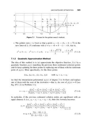
Figure 7.1 Process for the golden search method.

2
ž The golden ratio r is fixed so that a point c 1 = b 1 − rh 1 = b − r h in the
new interval [c, b] conforms with d = a + rh = b − (1 − r)h,thatis,
√ √
−1 + 1 + 4 −1 + 5
2 2
r = 1 − r, r + r − 1 = 0, r = = (7.1.3)
2 2
7.1.2 Quadratic Approximation Method
The idea of this method is to (a) approximate the objective function f(x) by a
quadratic function p 2 (x) matching the previous three (estimated solution) points
and (b) keep updating the three points by replacing one of them with the minimum
point of p 2 (x). More specifically, for the three points

{(x 0 ,f 0 ), (x 1 ,f 1 ), (x 2 ,f 2 )} with x 0 <x 1 <x 2

we find the interpolation polynomial p 2 (x) of degree 2 to fit them and replace

one of them with the zero of the derivative—that is, the root of p (x) = 0[see
2
Eq. (P3.1.2) in Problem 3.1]:
2
2
2
2
2
2
f 0 (x − x ) + f 1 (x − x ) + f 2 (x − x )
2
1
0
0
1
2
x = x 3 = (7.1.4)
2{f 0 (x 1 − x 2 ) + f 1 (x 2 − x 0 ) + f 2 (x 0 − x 1 )}
In particular, if the previous estimated solution points are equidistant with an
equal distance h (i.e., x 2 − x 1 = x 1 − x 0 = h), then this formula becomes
2 2 2 2 2 2
1
0
2
1
0
2
f 0 (x − x ) + f 1 (x − x ) + f 2 (x − x )
x 3 =
2{f 0 (x 1 − x 2 ) + f 1 (x 2 − x 0 ) + f 2 (x 0 − x 1 )} x 1 =x +h

x 2 =x 1 +h
3f 0 − 4f 1 + f 2
= x 0 + h (7.1.5)
2(−f 0 + 2f 1 − f 2 )