Page 329 - Applied Numerical Methods Using MATLAB

318 ORDINARY DIFFERENTIAL EQUATIONS
Substitutingthediscretizedboundarycondition(P6.11.11)into(P6.11.10)
yields
(P6.11.11a)
y −1 − 4y 0 + 6y 1 − 4y 2 + y 3 = λy 1 −−−−−→
5y 1 − 4y 2 + y 3 = λy 1
(P6.11.11a)
y 0 − 4y 1 + 6y 2 − 4y 3 + y 4 = λy 2 −−−−−→

− 4y 1 + 6y 2 − 4y 3 + y 4 = λy 2
y i − 4y i+1 + 6y i+2 − 4y i+3 + y i+4 = λy i+2
for i = 1: N − 5 (P6.11.12)
(P6.11.11b)
y N−4 − 4y N−3 + 6y N−2 − 4y N−1 + y N = λy N−2 −−−−−−→

y N−4 − 4y N−3 + 6y N−2 − 4y N−1 = λy N−2
(P6.11.11b)
y N−3 − 4y N−2 + 6y N−1 − 4y N + y N+1 = λy N−1 −−−−−−→

y N−3 − 4y N−2 + 5y N−1 = λy N−1
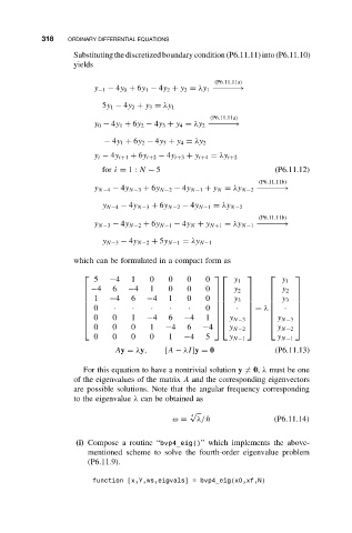
which can be formulated in a compact form as

5 −4 1 0 0 0 0 y 1 y 1
     
 −4 6 −4 1 0 0 0   y 2   y 2 
 1 −4 6 −4 1 0 0   y 3   


 
 y 3 
 0 · · · · · 0   ·   · 
 


 = λ 
 0 0 1 −4 6 −4 1   y N−3   

 

 y N−3 
0 0 0 1 −4 6 −4 y N−2 y N−2
     
0 0 0 0 1 −4 5 y N−1 y N−1
Ay = λy, [A − λI]y = 0 (P6.11.13)
For this equation to have a nontrivial solution y = 0, λ must be one
of the eigenvalues of the matrix A and the corresponding eigenvectors
are possible solutions. Note that the angular frequency corresponding
to the eigenvalue λ can be obtained as
√
4
ω = λ/h (P6.11.14)
(i) Compose a routine “bvp4_eig()” which implements the above-
mentioned scheme to solve the fourth-order eigenvalue problem
(P6.11.9).
function [x,Y,ws,eigvals] = bvp4_eig(x0,xf,N)