Page 327 - Applied Numerical Methods Using MATLAB

316 ORDINARY DIFFERENTIAL EQUATIONS

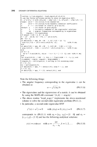
function [x,Y,ws,eigvals] = bvp2_eig(x0,xf,c0,cf,N)
% use the finite difference method to solve an eigenvalue BVP4:
% y"+w^2*y = 0 with c01y(x0) + c02y’(x0) = 0, cf1y(xf) + cf2y’(xf) = 0
%input: x0/xf = the initial/final boundaries
% c0/cf = the initial/final boundary condition coefficients
% N-1=the number of internal grid points.
%output: x = the vector of grid points
% Y = the matrix composed of the eigenvector solutions
% ws = angular frequencies corresponding to eigenvalues
% eigvals = the eigenvalues
if nargin < 5|N < 3, N = 3; end
h = (xf - x0)/N; h2 = h*h; x = x0+[0:N]*h;
N1=N+1;
if abs(c0(2)) < eps, N1 = N1 - 1; A(1,1:2) = [2 -1];
else A(1,1:2) = [2*(1-c0(1)/c0(2)*h) -2]; %(P6.11.4a)
end
if abs(cf(2)) < eps, N1 = N1 - 1; A(N1,N1 - 1:N1) = [-1 2];
else A(N1,N1 - 1:N1) = [-2 2*(1 + cf(1)/cf(2)*h)]; %(P6.11.4c)
end
if N1 > 2
for m = 2:ceil(N1/2), A(m,m - 1:m + 1) = [-1 2 -1]; end %(P6.11.4b)
end
for m=ceil(N1/2) + 1:N1 - 1, A(m,:) = fliplr(A(N1+1- m,:)); end
[V,LAMBDA] = eig(A); eigvals = diag(LAMBDA)’;
[eigvals,I] = sort(eigvals); % sorting in the ascending order
V = V(:,I);
ws = sqrt(eigvals)/h;
if abs(c0(2)) < eps, Y = zeros(1,N1); else Y = []; end
Y = [Y; V];
if abs(cf(2)) < eps, Y = [Y; zeros(1,N1)]; end

Note the following things:
ž The angular frequency corresponding to the eigenvalue λ can be
obtained as

ω = λ/a 0 /h (P6.11.6)
ž The eigenvalues and the eigenvectors of a matrix A can be obtained
by using the MATLAB command ‘[V,D] = eig(A)’.
ž The above routine “bvp2_eig()” implements the above-mentioned
scheme to solve the second-order eigenvalue problem (P6.11.1).
ž In particular, a second-order eigenvalue BVP

2

y (x) + ω y = 0 with y(x 0 ) = 0,y(x f ) = 0 (P6.11.7)
corresponds to (P6.11.1) with c 0 = [c 01 c 02 ] = [1 0] and c f =
[c f 1 c f 2 ] = [1 0] and has the following analytical solutions:

kπ
y(x) = a sin ωx with ω = ,k = 1, 2,. .. (P6.11.8)
x f − x 0