Page 324 - Applied Numerical Methods Using MATLAB

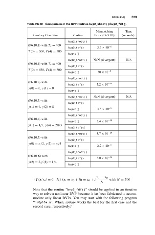
PROBLEMS 313
Table P6.10 Comparison of the BVP routines bvp2 shoot()/bvp2 fdf()

Mismatching Time
Boundary Condition Routine Error (P6.9.0b) (seconds)
bvp2 shoot()
(P6.10.1) with T a = 400
bvp2 fdf() 3.6 × 10 −6
T(0) = 500, T(4) = 300
bvp4c()
bvp2 shoot() NaN (divergent) N/A
(P6.10.1) with T a = 400
bvp2 fdf()
T(0) = 550, T(4) = 300 −5
bvp4c() 30 × 10
bvp2 shoot()
(P6.10.2) with −13
bvp2 fdf() 3.2 × 10
y(0) = 0, y(1) = 0
bvp4c()
bvp2 shoot() NaN (divergent) N/A
(P6.10.3) with
bvp2 fdf()
y(1) = 4, y(2) = 8
bvp4c() 3.5 × 10 −6
bvp2 shoot()
(P6.10.4) with
bvp4c() 3.4 × 10 −10
y(1) = 1/3, y(4) = 20/3
bvp2 fdf(c)
bvp2 shoot() 3.7 × 10 −14
(P6.10.5) with
bvp2 fdf()
y(0) = π/2, y(2) = π/4 −9
bvp4c() 2.2 × 10

bvp2 shoot()
(P6.10-6) with −14
bvp2 fdf() 5.0 × 10
y(2) = 2,y (8) = 1/4

bvp4c()

x f − x 0
{T(x i ), i = 0: N} (x i = x 0 + ih = x 0 + i with N = 500
N
Note that the routine “bvp2_fdf()” should be applied in an iterative
way to solve a nonlinear BVP, because it has been fabricated to accom-
modate only linear BVPs. You may start with the following program
“nm6p10a.m”. Which routine works the best for the first case and the
second case, respectively?