Page 321 - Applied Numerical Methods Using MATLAB

310 ORDINARY DIFFERENTIAL EQUATIONS

%nm6p08a.m: to solve BVP2 with mixed boundary conditions
%x" = (2t/t^2 + 1)*x’ -2/(t^2+1)*x +t^2+1
% with x(0)+6x’(0) = 0, x’(1) + x(1) = 0
%shooting method
f = inline(’[x(2); 2*(t*x(2) - x(1))./(t.^2 + 1)+(t.^2 + 1)]’,’t’,’x’);
t0 = 0; tf = 1; N = 100; tol = 1e-8; kmax = 10;
c0 = [1 6 0]; cf = [1 1 0]; %coefficient vectors of boundary condition
[tt,x_sh] = bvp2mm_shoot(f,t0,tf,c0,cf,N,tol,kmax);
plot(tt,x_sh(:,1),’b’)
%nm6p08b.m: finite difference method
a1 = inline(’-2*t./(t.^2+1)’,’t’); a0 = inline(’2./(t.^2+1)’,’t’);
u = inline(’t.^2+1’,’t’);
t0 = 0; tf = 1; N = 500;
c0 = [1 6 0]; cf = [1 1 0]; %coefficient vectors of boundary condition
[tt,x_fd] = bvp2mm_fdf(a1,a0,u,t0,tf,c0,cf,N);
plot(tt,x_fd,’r’)

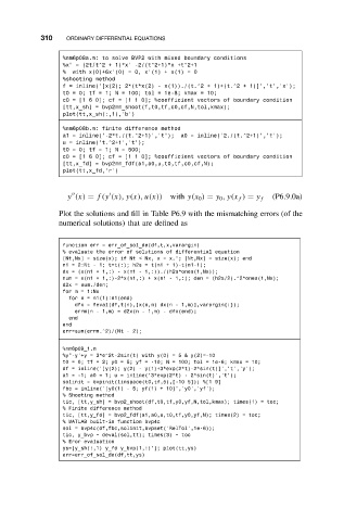
y (x) = f(y (x), y(x), u(x)) with y(x 0 ) = y 0 ,y(x f ) = y f (P6.9.0a)

Plot the solutions and fill in Table P6.9 with the mismatching errors (of the
numerical solutions) that are defined as

function err = err_of_sol_de(df,t,x,varargin)
% evaluate the error of solutions of differential equation
[Nt,Nx] = size(x); if Nt < Nx, x = x.’; [Nt,Nx] = size(x); end
n1 = 2:Nt - 1; t=t(:); h2s = t(n1 + 1)-t(n1-1);
dx = (x(n1 + 1,:) - x(n1 - 1,:))./(h2s*ones(1,Nx));
num = x(n1 + 1,:)-2*x(n1,:) + x(n1 - 1,:); den = (h2s/2).^2*ones(1,Nx);
d2x = num./den;
for m = 1:Nx
for n = n1(1):n1(end)
dfx = feval(df,t(n),[x(n,m) dx(n - 1,m)],varargin{:});
errm(n - 1,m) = d2x(n - 1,m) - dfx(end);
end
end
err=sum(errm.^2)/(Nt - 2);
%nm6p09_1.m
%y"-y’+y = 3*e^2t-2sin(t) with y(0)=5& y(2)=-10
t0 = 0; tf = 2; y0 = 5; yf = -10; N = 100; tol = 1e-6; kmax = 10;
df = inline(’[y(2); y(2) - y(1)+3*exp(2*t)-2*sin(t)]’,’t’,’y’);
a1 = -1; a0 = 1; u = inline(’3*exp(2*t) - 2*sin(t)’,’t’);
solinit = bvpinit(linspace(t0,tf,5),[-10 5]); %[1 9]
fbc = inline(’[y0(1) - 5; yf(1) + 10]’,’y0’,’yf’);
% Shooting method
tic, [tt,y_sh] = bvp2_shoot(df,t0,tf,y0,yf,N,tol,kmax); times(1) = toc;
% Finite difference method
tic, [tt,y_fd] = bvp2_fdf(a1,a0,u,t0,tf,y0,yf,N); times(2) = toc;
% MATLAB built-in function bvp4c
sol = bvp4c(df,fbc,solinit,bvpset(’RelTol’,1e-6));
tic, y_bvp = deval(sol,tt); times(3) = toc
% Eror evaluation
ys=[y_sh(:,1) y_fd y_bvp(1,:)’]; plot(tt,ys)
err=err_of_sol_de(df,tt,ys)