Page 318 - Applied Numerical Methods Using MATLAB

PROBLEMS 307
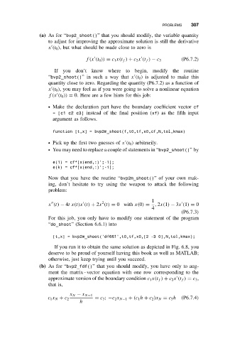
(a) As for “bvp2_shoot()” that you should modify, the variable quantity
to adjust for improving the approximate solution is still the derivative

x (t 0 ), but what should be made close to zero is

f(x (t 0 )) = c 1 x(t f ) + c 2 x (t f ) − c 3 (P6.7.2)
If you don’t know where to begin, modify the routine

“bvp2_shoot()”insuchawaythat x (t 0 ) is adjusted to make this
quantity close to zero. Regarding the quantity (P6.7.2) as a function of

x (t 0 ), you may feel as if you were going to solve a nonlinear equation

f(x (t 0 )) = 0. Here are a few hints for this job:
ž Make the declaration part have the boundary coefficient vector cf
= [c1 c2 c3] instead of the final position (xf) as the fifth input
argument as follows.

function [t,x] = bvp2m_shoot(f,t0,tf,x0,cf,N,tol,kmax)
ž Pick up the first two guesses of x (t 0 ) arbitrarily.

ž You may need to replace a couple of statements in “bvp2_shoot()”by

e(1) = cf*[x(end,:)’;-1];
e(k) = cf*[x(end,:)’;-1];

Now that you have the routine “bvp2m_shoot()” of your own mak-
ing, don’t hesitate to try using the weapon to attack the following
problem:
1
2
x (t) − 4t x(t)x (t) + 2x (t) = 0 with x(0) = , 2x(1) − 3x (1) = 0
4
(P6.7.3)
For this job, you only have to modify one statement of the program
“do_shoot” (Section 6.6.1) into

[t,x] = bvp2m_shoot(’df661’,t0,tf,x0,[2 -3 0],N,tol,kmax);

If you run it to obtain the same solution as depicted in Fig. 6.8, you
deserve to be proud of yourself having this book as well as MATLAB;
otherwise, just keep trying until you succeed.
(b) As for “bvp2_fdf()” that you should modify, you have only to aug-
ment the matrix–vector equation with one row corresponding to the
approximate version of the boundary condition c 1 x(t f ) + c 2 x (t f ) = c 3 ,

that is,
x N − x N−1
c 1 x N + c 2 = c 3 ; −c 2 x N−1 + (c 1 h + c 2 )x N = c 3 h(P6.7.4)
h