Page 323 - Applied Numerical Methods Using MATLAB

312 ORDINARY DIFFERENTIAL EQUATIONS
Overall, which routine works the best for linear BVPs among the three
routines?

(a) y (x) = y (x) − y(x) + 3e 2x − 2sin x with y(0) = 5,y(2) =−10
(P6.9.1)

(b) y (x) =−4y(x) with y(0) = 5,y(1) =−5 (P6.9.2)
2
−7
−6

(c) y (t) = 10 y(t) + 10 (t − 50t) with y(0) = 0,y(50) = 0 (P6.9.3)

(d) y (t) =−2y(t) + sin t with y(0) = 0,y(1) = 0 (P6.9.4)
x

(e) y (x) = y (x) + y(x) + e (1 − 2x) with y(0) = 1,y(1) = 3e (P6.9.5)

2
d y(r) 1 dy(r)
(f) + = 0 with y(1) = ln 1,y(2) = ln 2 (P6.9.6)
dr 2 r dr
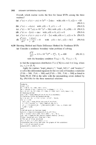
6.10 Shooting Method and Finite Difference Method for Nonlinear BVPs
(a) Consider a nonlinear boundary value problem of solving
2
d T −9 4 4
= 1.9 × 10 (T − T ), T a = 400 (P6.10.1)
a
dx 2
with the boundary condition T(x 0 ) = T 0 ,T (x f ) = T f
◦
to find the temperature distribution T(x) [ K] in a rod 4 m long, where
[x 0 ,x f ] = [0, 4].
Apply the routines “bvp2_shoot()”, “bvp2_fdf()”, and “bvp4c()”
to solve this differential equation for the two sets of boundary conditions
{T(0) = 500,T (4) = 300} and {T(0) = 550,T (4) = 300} as listed in
Table P6.10. Fill in the table with the mismatching errors defined by
Eq. (P6.9.0b) for the three numerical solutions
%nm6p10a
clear, clf
K = 1.9e-9; Ta = 400; Ta4 = Ta^4;
df = inline(’[T(2); 1.9e-9*(T(1).^4-256e8)]’,’t’,’T’);
x0 = 0; xf = 4; T0 = 500; Tf = 300; N = 500; tol = 1e-5; kmax = 10;
% Shooting method
[xx,T_sh] = bvp2_shoot(df,x0,xf,T0,Tf,N,tol,kmax);
% Iterative finite difference method
a1 = 0; a0 = 0; u = T0 + [1:N - 1]*(Tf - T0)/N;
for i = 1:100
[xx,T_fd] = bvp2_fdf(a1,a0,u,x0,xf,T0,Tf,N);
u = K*(T_fd(2:N).^4 - Ta4); %RHS of (P6.10.1)
ifi>1& norm(T_fd - T_fd0)/norm(T_fd0) < tol, i, break; end
T_fd0 = T_fd;
end
% MATLAB built-in function bvp4c
solinit = bvpinit(linspace(x0,xf,5),[Tf T0]);
fbc = inline(’[Ta(1)-500; Tb(1)-300]’,’Ta’,’Tb’);
tic, sol = bvp4c(df,fbc,solinit,bvpset(’RelTol’,1e-6));
T_bvp = deval(sol,xx); time_bvp = toc;
% The set of three solutions
Ts = [T_sh(:,1) T_fd T_bvp(1,:)’];
% Evaluates the errors and plot the graphs of the solutions
err = err_of_sol_de(df,xx,ys)
subplot(321), plot(xx,Ts)