Page 326 - Applied Numerical Methods Using MATLAB

PROBLEMS 315
with
y 1 − y −1 c 01
c 01 y 0 + c 02 = 0 → y −1 = 2h y 0 + y 1 (P6.11.3a)
2h c 02
y N+1 − y N−1 c f 1
c f 1 y N + c f 2 = 0 → y N+1 = y N−1 − 2h y N
2h c f 2
(P6.11.3b)
Substituting the discretized boundary condition (P6.11.3) into (P6.11.2)
yields
(P6.11.3a)
y −1 − 2y 0 + y 1 =−λy 0 −−−−−→

c 01
2 − 2h y 0 − 2y 1 = λy 0 (P6.11.4a)
c 02
y i−1 − 2y i + y i+1 =−λy i →−y i−1 + 2y i − y i+1 = λy i
for i = 1: N − 1 (P6.11.4b)
(P6.11.3b)
y N−1 − 2y N + y N+1 =−λy N −−−−−→

c f 1
− 2y N−1 + 2 + 2h y N = λy N (P6.11.4c)
c f 2
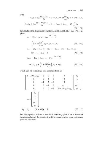
which can be formulated in a compact form as

 −2 0 0 0   
2 − 2hc 01 /c 02 y 0
−1 2 −1 0 0
   
   y 1 
0 −1 2 −1 0 ·
   
   
   
0 0 −1 2 −1
   y N−1 
0 0 0 −2 2 + 2hc f 1 /c f 2 y N
 
y 0
 
 y 1 
 
·
= λ  
 
 y N−1 
y N
Ay = λy; [A − λI]y = 0 (P6.11.5)
For this equation to have a nontrivial solution y = 0, λ must be one of
the eigenvalues of the matrix A and the corresponding eigenvectors are
possible solutions.