Page 328 - Applied Numerical Methods Using MATLAB

PROBLEMS 317
0.1 0.1

0.05 0.05

0 0

−0.05 −0.05

−0.1 −0.1
0 0.5 1 1.5 2 0 0.5 1 1.5 2
(a) Eigenvector solutions for BVP2 (b) Eigenvector solutions for BVP4
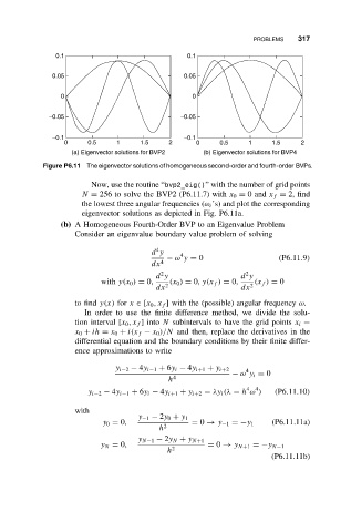
Figure P6.11 The eigenvector solutions of homogeneous second-order and fourth-order BVPs.
Now, use the routine “bvp2_eig()” with the number of grid points
N = 256 to solve the BVP2 (P6.11.7) with x 0 = 0and x f = 2, find
the lowest three angular frequencies (ω i ’s) and plot the corresponding
eigenvector solutions as depicted in Fig. P6.11a.
(b) A Homogeneous Fourth-Order BVP to an Eigenvalue Problem
Consider an eigenvalue boundary value problem of solving

4
d y 4
− ω y = 0 (P6.11.9)
dx 4
2
2
d y d y
with y(x 0 ) = 0, (x 0 ) = 0,y(x f ) = 0, (x f ) = 0
dx 2 dx 2
to find y(x) for x ∈ [x 0 ,x f ] with the (possible) angular frequency ω.
In order to use the finite difference method, we divide the solu-
tion interval [x 0 ,x f ]into N subintervals to have the grid points x i =
x 0 + ih = x 0 + i(x f − x 0 )/N and then, replace the derivatives in the
differential equation and the boundary conditions by their finite differ-
ence approximations to write

y i−2 − 4y i−1 + 6y i − 4y i+1 + y i+2 4
− ω y i = 0
h 4
4
4
y i−2 − 4y i−1 + 6y i − 4y i+1 + y i+2 = λy i (λ = h ω ) (P6.11.10)
with
y −1 − 2y 0 + y 1
y 0 = 0, = 0 → y −1 =−y 1 (P6.11.11a)
h 2
y N−1 − 2y N + y N+1
y N = 0, = 0 → y N+1 =−y N−1
h 2
(P6.11.11b)