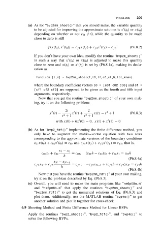
Page 320 - Applied Numerical Methods Using MATLAB

PROBLEMS 309
(a) As for “bvp2mm_shoot()” that you should make, the variable quantity
to be adjusted for improving the approximate solution is x (t 0 ) or x(t 0 )

depending on whether or not c 01 = 0, while the quantity to be made
close to zero is still

f(x(t 0 ), x (t 0 )) = c f 1 x(t f ) + c f 2 x (t f ) − c f 3 (P6.8.2)
If you don’t have your own idea, modify the routine “bvp2m_shoot()”

in such a way that x (t 0 ) or x(t 0 ) is adjusted to make this quantity

close to zero and x(t 0 ) or x (t 0 ) is set by (P6.8.1a), making its decla-
ration as
function [t,x] = bvp2mm_shoot(f,t0,tf,c0,cf,N,tol,kmax)

where the boundary coefficient vectors c0 = [c01 c02 c03] and cf =
[cf1 cf2 cf3] are supposed to be given as the fourth and fifth input
arguments, respectively.
Now that you get the routine “bvp2mm_shoot()” of your own mak-
ing, try it on the following problem:

2t 2
2
x (t) − x (t) + x(t) = t + 1 (P6.8.3)
2
2
t + 1 t + 1

with x(0) + 6x (0) = 0,x(1) + x (1) = 0
(b) As for “bvp2_fdf()” implementing the finite difference method, you
only have to augment the matrix–vector equation with two rows
corresponding to the approximate versions of the boundary conditions

c 01 x(t 0 ) + c 02 x (t 0 ) = c 03 and c f 1 x(t f ) + c f 2 x (t f ) = c f 3 ,thatis,
x 1 − x 0
c 01 x 0 + c 02 = c 03 , (c 01 h − c 02 )x 0 + c 02 x 1 = c 03 h
h
(P6.8.4a)
x N − x N−1
c f 1 x N + c f 2 = c f 3 ; −c f 2 x N−1 + (c f 1 h + c f 2 )x N = c f 3 h
h
(P6.8.4b)
Now that you have the routine “bvp2mm_fdf()” of your own making,
try it on the problem described by Eq. (P6.8.3).
(c) Overall, you will need to make the main programs like “nm6p08a.m”
and “nm6p08b.m” that apply the routines “bvp2mm_shoot()”and
“bvp2mm_fdf()” to get the numerical solutions of Eq. (P6.8.3) and
plot them. Additionally, use the MATLAB routine “bvp4c()”to get
another solution and plot it together for cross-check.
6.9 Shooting Method and Finite Difference Method for Linear BVPs

Apply the routines “bvp2_shoot()”, “bvp2_fdf()”, and “bvp4c()”to
solve the following BVPs.