Page 316 - Applied Numerical Methods Using MATLAB

PROBLEMS 305

× 10 7
6
× × × × × × × ×
× ×
x 2 × × × ×
× ×
× × × × × × ×
4 × × × × × ×
× ×
× × ×
× × × ×
× ×
× × ×
× × × × ×× ×
2 × × × × ×× ×× × × × ×
× × × × × × × × ×
× × × × × × × ×
× × × × × × × ×
× × × × × × × × × ×
× × × × × × × × ×
0 × × × × Earth × ×
× × × × × × × × × ×
× × × × × × × × × × × ×
× × × × × × × × ×
× × × × × × ×
× × × × × × ×
−2 × × × × × × × × × × × × × × × × × × × × × × ×
× ×
× × × × ×
× ×
ode_RK4( )
× ×
ode45( ) ×
× ×
−4 ×××× ode23s( ) × × × × × × × × × ×
−8 −6 −4 −2 0 2 x 1 4 × 10 7
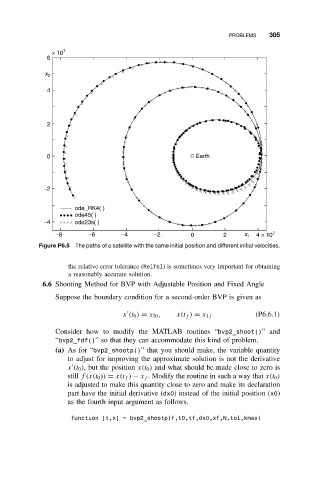
Figure P6.5 The paths of a satellite with the same initial position and different initial velocities.
the relative error tolerance (RelTol) is sometimes very important for obtaining
a reasonably accurate solution.
6.6 Shooting Method for BVP with Adjustable Position and Fixed Angle
Suppose the boundary condition for a second-order BVP is given as

x (t 0 ) = x 20 , x(t f ) = x 1f (P6.6.1)
Consider how to modify the MATLAB routines “bvp2_shoot()”and
“bvp2_fdf()” so that they can accommodate this kind of problem.
(a) As for “bvp2_shootp()” that you should make, the variable quantity
to adjust for improving the approximate solution is not the derivative
x (t 0 ), but the position x(t 0 ) and what should be made close to zero is

still f(x(t 0 )) = x(t f ) − x f . Modify the routine in such a way that x(t 0 )
is adjusted to make this quantity close to zero and make its declaration
part have the initial derivative (dx0) instead of the initial position (x0)
as the fourth input argument as follows.

function [t,x] = bvp2_shootp(f,t0,tf,dx0,xf,N,tol,kmax)