Page 311 - Applied Numerical Methods Using MATLAB

300 ORDINARY DIFFERENTIAL EQUATIONS
(ii) If we apply the Laplace transform technique to solve this equation
with zero initial condition i(0) = 0, we can get

I 1 (s) (6.5.5) −1
I 2 (s) = [sI − A] Bu(s)
−1
s + G 1 /C 1 G 1 /C 2 G 1 1
=
G 1 /C 2 s + (G 1 + G 2 )/C 2 G 1 s
G 1
I 2 (s) =
2
s + (G 1 /C 1 + (G 1 + G 2 )/C 2 )s + G 1 G 2 /C 1 C 2
1/100
=
2
s + 2100s + 100000
1/100
∼
=
(s + 2051.25)(s + 48.75)
1 1 1
∼
= −
200250 s + 48.75 s + 2051.25
1
∼ −48.75t −2051.25t
i 2 (t) = (e − e ) (P6.3.7e)
200250
where λ 1 =−2051.25 and λ 2 =−48.75 are actually the eigenval-
ues of the system matrix A in Eq. (P6.3.7d). Find the measure of
stiffness defined by Eq. (6.5.26).
(iii) Using the MATLAB symbolic computation command “dsolve()”,
find the analytical solution of the differential equation (P6.3.7b) and
plot i 2 (t) together with (P6.3.7e) for 0 ≤ t ≤ 0.05 s. Which of the
two numerical solutions obtained in (i) is better? You may refer to
the following code:

syms R1 R2 C1 C2
i = dsolve(’(R1+R2)*Di1 - R2*Di2 + i1/C1 = 1’,...
’-R2*Di1 + R2*Di2 + i2/C2’,’i1(0) = 0’,’i2(0) = 0’); %(P6.3.7b)
R1 = 100; R2 = 1000; C1 = 1e-5; C2 = 1e-5;
t0 = 0; tf = 0.05; t = t0+(tf-t0)/100*[0:100];
i2t = eval(i.i2); plot(t,i2t,’m’)

6.4 Physical Meaning of a Solution for Differential Equation and Its Animation

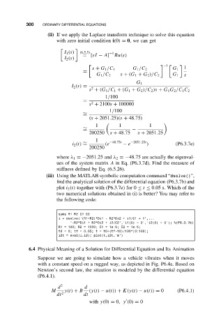
Suppose we are going to simulate how a vehicle vibrates when it moves
with a constant speed on a rugged way, as depicted in Fig. P6.4a. Based on
Newton’s second law, the situation is modeled by the differential equation
(P6.4.1).

d 2 d
M y(t) + B (y(t) − u(t)) + K(y(t) − u(t)) = 0 (P6.4.1)
dt 2 dt

with y(0) = 0,y (0) = 0