Page 309 - Applied Numerical Methods Using MATLAB

298 ORDINARY DIFFERENTIAL EQUATIONS
w
loop filter c
u(t) = sin(w t) a x (t)
1
o
y(t)
1 + τs
x (t) 1
2
oscillator
cos(x (t)) s
2
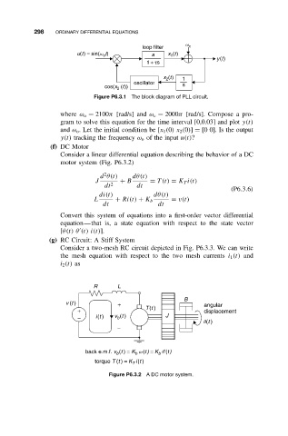
Figure P6.3.1 The block diagram of PLL circuit.
where ω o = 2100π [rad/s] and ω c = 2000π [rad/s]. Compose a pro-
gram to solve this equation for the time interval [0,0.03] and plot y(t)
and ω o . Let the initial condition be [x 1 (0)x 2 (0)] = [0 0]. Is the output
y(t) tracking the frequency ω o of the input u(t)?
(f) DC Motor
Consider a linear differential equation describing the behavior of a DC
motor system (Fig. P6.3.2)

2
d θ(t) dθ(t)
J + B = T(t) = K T i(t)
dt 2 dt
(P6.3.6)
di(t) dθ(t)
L + Ri(t) + K b = v(t)
dt dt
Convert this system of equations into a first-order vector differential
equation—that is, a state equation with respect to the state vector
[θ(t) θ (t) i(t)].

(g) RC Circuit: A Stiff System
Consider a two-mesh RC circuit depicted in Fig. P6.3.3. We can write
the mesh equation with respect to the two mesh currents i 1 (t) and
i 2 (t) as

R L

B
v (t ) + angular
+ T(t ) displacement
− i(t ) v (t ) J
b
q(t )
−

back e.m.f. v (t ) = K w(t) = K q'(t)
b
b
b
torque T (t ) = K i(t )
T
Figure P6.3.2 A DC motor system.