Page 305 - Applied Numerical Methods Using MATLAB

294 ORDINARY DIFFERENTIAL EQUATIONS

0.5

0

−0.5
2
3
1 1 2
0 0
−1
−1 −2
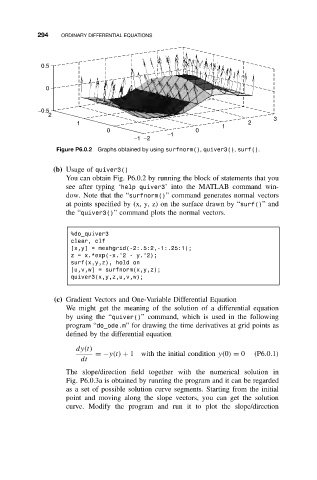
Figure P6.0.2 Graphs obtained by using surfnorm(), quiver3(), surf().

(b) Usage of quiver3()
You can obtain Fig. P6.0.2 by running the block of statements that you
see after typing ‘help quiver3’ into the MATLAB command win-
dow. Note that the “surfnorm()” command generates normal vectors
at points specified by (x, y, z) on the surface drawn by “surf()”and
the “quiver3()” command plots the normal vectors.

%do_quiver3
clear, clf
[x,y] = meshgrid(-2:.5:2,-1:.25:1);
z = x.*exp(-x.^2 - y.^2);
surf(x,y,z), hold on
[u,v,w] = surfnorm(x,y,z);
quiver3(x,y,z,u,v,w);

(c) Gradient Vectors and One-Variable Differential Equation
We might get the meaning of the solution of a differential equation
by using the “quiver()” command, which is used in the following
program “do_ode.m” for drawing the time derivatives at grid points as
defined by the differential equation

dy(t)
=−y(t) + 1 with the initial condition y(0) = 0 (P6.0.1)
dt
The slope/direction field together with the numerical solution in
Fig. P6.0.3a is obtained by running the program and it can be regarded
as a set of possible solution curve segments. Starting from the initial
point and moving along the slope vectors, you can get the solution
curve. Modify the program and run it to plot the slope/direction