Page 303 - Applied Numerical Methods Using MATLAB

292 ORDINARY DIFFERENTIAL EQUATIONS

%do_fdf to solve BVP2 by the finite difference method
clear, clf
t0 = 1; x0 = 5; tf = 2; xf = 3; N = 100;
a1 = inline(’2./t’,’t’); a0 = inline(’-2./t./t’,’t’); u = 0; %Eq.(6.6.10)
[tt,x] = bvp2_fdf(a1,a0,u,t0,tf,x0,xf,N);
%use the MATLAB built-in command ’bvp4c()’
df = inline(’[x(2); 2./t.*(x(1)./t - x(2))]’,’t’,’x’);
fbc = inline(’[x0(1) - 5; xf(1) - 3]’,’x0’,’xf’);
solinit = bvpinit(linspace(t0,tf,5),[1 10]); %initial solution interval
sol = bvp4c(df,fbc,solinit,bvpset(’RelTol’,1e-4));
x_bvp = deval(sol,tt); xbv = x_bvp(1,:)’;
%use the symbolic computation command ’dsolve()’
xo = dsolve(’D2x + 2*(Dx - x/t)/t=0’,’x(1) = 5, x(2) = 3’)
xot = subs(xo,’t’,tt); %xot=4./tt./tt +tt; %true analytical solution
err_fd = norm(x - xot)/(N+1) %error between numerical/analytical solution
err_bvp = norm(xbv - xot)/(N + 1)
plot(tt,x,’b’,tt,xbv,’r’,tt,xot,’k’) %compare with analytical solution

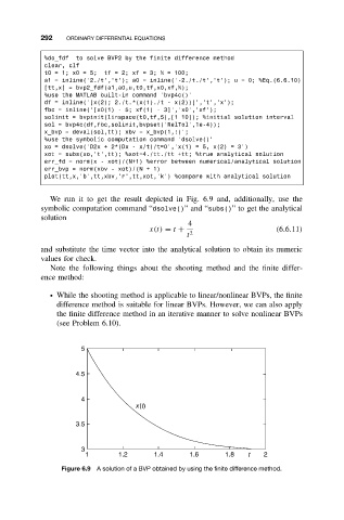
We run it to get the result depicted in Fig. 6.9 and, additionally, use the
symbolic computation command “dsolve()”and “subs()” to get the analytical
solution
4
x(t) = t + (6.6.11)
t 2
and substitute the time vector into the analytical solution to obtain its numeric
values for check.
Note the following things about the shooting method and the finite differ-
ence method:

ž While the shooting method is applicable to linear/nonlinear BVPs, the finite
difference method is suitable for linear BVPs. However, we can also apply
the finite difference method in an iterative manner to solve nonlinear BVPs
(see Problem 6.10).

5

4.5

4
x(t)

3.5

3
1 1.2 1.4 1.6 1.8 t 2
Figure 6.9 A solution of a BVP obtained by using the finite difference method.