Page 299 - Applied Numerical Methods Using MATLAB

288 ORDINARY DIFFERENTIAL EQUATIONS

of x (t 0 ) and solving the IVP repetitively until the final value x(t f ) of the solution
matches the given boundary value x f with enough accuracy. It is similar to
adjusting the angle of firing a cannon so that the shell will eventually hit the target
and that’s why this method is named the shooting method. This can be viewed

as a nonlinear equation problem, if we regard x (t 0 ) as an independent variable
and the difference between the resulting final value x(t f ) and the desired one x f
as a (mismatching) function of x (t 0 ). So the solution scheme can be systemized

by using the secant method (Section 4.5) and is cast into the MATLAB routine
“bvp2_shoot()”.

(cf) We might have to adjust the shooting position with the angle fixed, instead of adjust-
ing the shooting angle with the position fixed or deal with the mixed-boundary
conditions. See Problems 6.6, 6.7, and 6.8.

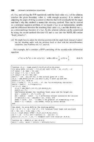
For example, let’s consider a BVP consisting of the second-order differential
equation

1 1
2

x (t) = 2x (t) + 4t x(t)x (t) with x(0) = ,x(1) = (6.6.3)
4 3
function [t,x] = bvp2_shoot(f,t0,tf,x0,xf,N,tol,kmax)
%To solve BVP2: [x1,x2]’ = f(t,x1,x2) with x1(t0) = x0, x1(tf) = xf
if nargin < 8, kmax = 10; end
if nargin < 7, tol = 1e-8; end
if nargin < 6, N = 100; end
dx0(1) = (xf - x0)/(tf-t0); % the initial guess of x’(t0)
[t,x] = ode_RK4(f,[t0 tf],[x0 dx0(1)],N); % start up with RK4
plot(t,x(:,1)), hold on
e(1) = x(end,1) - xf; % x(tf) - xf: the 1st mismatching (deviation)
dx0(2) = dx0(1) - 0.1*sign(e(1));
fork=2: kmax-1
[t,x] = ode_RK4(f,[t0 tf],[x0 dx0(k)],N);
plot(t,x(:,1))
%difference between the resulting final value and the target one
e(k) = x(end,1) - xf; % x(tf)- xf
ddx = dx0(k) - dx0(k - 1); % difference between successive derivatives
if abs(e(k))< tol | abs(ddx)< tol, break; end
deddx = (e(k) - e(k - 1))/ddx; % the gradient of mismatching error
dx0(k + 1) = dx0(k) - e(k)/deddx; %move by secant method
end
%do_shoot to solve BVP2 by the shooting method
t0 = 0; tf = 1; x0 = 1/4; xf = 1/3; %initial/final times and positions
N = 100; tol = 1e-8; kmax = 10;
[t,x] = bvp2_shoot(’df661’,t0,tf,x0,xf,N,tol,kmax);
xo = 1./(4 - t.*t); err = norm(x(:,1) - xo)/(N + 1)
plot(t,x(:,1),’b’, t,xo,’r’) %compare with true solution (6.6.4)
function dx = df661(t,x) %Eq.(6.6.5)
dx(1) = x(2); dx(2) = (2*x(1) + 4*t*x(2))*x(1);