Page 295 - Applied Numerical Methods Using MATLAB

284 ORDINARY DIFFERENTIAL EQUATIONS
called an IVP (Initial Value Problem):

(2)

[IVP] N : x (N) (t) = f(t, x(t),x (t), x (t), ...,x (N−1) (t))
(6.5.22)

with the initial values x(t 0 ) = x 10 ,x (t 0 ) = x 20 ,..., x (N−1) (t 0 ) = x N0
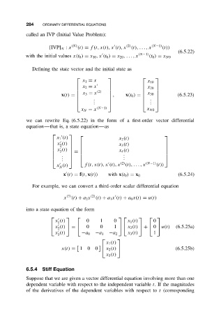
Defining the state vector and the initial state as

x 1 = x x 10
   
 x 2 = x   x 20 
 (2)   
 x 3 = x   x 30 
 , (6.5.23)
x(t) =  x(t 0 ) =  
.
.
   . 
.
 .   . 
x N = x (N−1) x N0
we can rewrite Eq. (6.5.22) in the form of a first-order vector differential
equation—that is, a state equation—as
 

x 1 (t)  x 2 (t) 

x (t)
2  
  x 3 (t)
 
 
3  =  
 x (t)  x 4 (t)
.  
 .
.  . 
  .
 . 
(2)

x (t) f(t, x(t), x (t), x (t), ...,x (N−1) (t))

N

x (t) = f(t, x(t)) with x(t 0 ) = x 0 (6.5.24)
For example, we can convert a third-order scalar differential equation
(2)
(3)

x (t) + a 2 x (t) + a 1 x (t) + a 0 x(t) = u(t)
into a state equation of the form
       
x (t) 0 1 0 x 1 (t) 0
1

2
 x (t)  =  0 0 1   x 2 (t)  +  0  u(t) (6.5.25a)

x (t) −a 0 −a 1 −a 2 x 3 (t) 1
3
 
x 1 (t)

x(t) = 10 0  x 2 (t)  (6.5.25b)
x 3 (t)
6.5.4 Stiff Equation
Suppose that we are given a vector differential equation involving more than one
dependent variable with respect to the independent variable t. If the magnitudes
of the derivatives of the dependent variables with respect to t (corresponding