Page 296 - Applied Numerical Methods Using MATLAB

VECTOR DIFFERENTIAL EQUATIONS 285
to their changing rates) are significantly different, such a differential equation is
said to be stiff because it is difficult to be solved numerically. For such a stiff
differential equation, we should be very careful in choosing the step-size in order
to avoid numerical instability problem and get a reasonably accurate solution
within a reasonable computation time. Why? Because we should use a small
step-size to grasp rapidly changing variables, and it requires a lot of computation
to cover slowly changing variables for such a long time as it lasts.
Actually, there is no clear distinction between stiff and non-stiff differential
equations, since stiffness of a differential equation is a matter of degree. Then, is
there any way to estimate the degree of stiffness for a given differential equation?
The answer is yes, if the differential equation can be arranged into an LTI state
equation like Eq. (6.5.4), the solution of which consists of components having
the time constants (modes) equal to the eigenvalues of the system matrix A.For
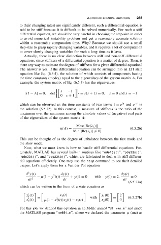
example, the system matrix of Eq. (6.5.3) has the eigenvalues

s −1
|sI − A|= 0, det = s(s + 1) = 0, s = 0and s =−1
0 s + 1
which can be observed as the time constants of two terms 1 = e 0t and e −t in
the solution (6.5.12). In this context, a measure of stiffness is the ratio of the
maximum over the minimum among the absolute values of (negative) real parts
of the eigenvalues of the system matrix A:
Max{|Re(λ i )|}
η(A) = (6.5.26)
Min{|Re(λ i )| = 0}

This can be thought of as the degree of unbalance between the fast mode and
the slow mode.
Now, what we must know is how to handle stiff differential equations. For-
tunately, MATLAB has several built-in routines like “ode15s()”, “ode23s()”,
“ode23t()”, and “ode23tb()”, which are fabricated to deal with stiff differen-
tial equations efficiently. One may use the help command to see their detailed
usages. Let’s apply them for a Van der Pol equation
2
d y(t) 2 dy(t) dy(t)
− µ(1 − y (t)) + y(t) = 0 with y(0) = 2, = 0
dt 2 dt dt
(6.5.27a)
which can be written in the form of a state equation as

x (t) x 2 (t) x 1 (0) 2
1 = with = (6.5.27b)
2

x (t) µ(1 − x (t))x 2 (t) − x 1 (t) x 2 (0) 0
2 1
For this job, we defined this equation in an M-file named “df_van.m” and made
the MATLAB program “nm654.m”, where we declared the parameter µ (mu) as