Page 294 - Applied Numerical Methods Using MATLAB

VECTOR DIFFERENTIAL EQUATIONS 283
1.5

1 x [n]
1
x (t)
0.5 1

x (t)
0 2
continuous-time
x [n]
2
−0.5 T = 0.05
T = 0.2
−1
0 0.5 1 1.5 2
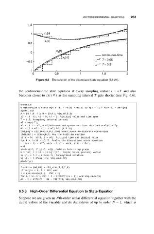
Figure 6.6 The solution of the discretized state equation (6.5.21).

the continuous-time state equation at every sampling instant t = nT and also
becomes closer to x(t) ∀ t as the sampling interval T gets shorter (see Fig. 6.6).

%nm652.m
% discretize a state eqn x’(t) = Ax(t) + Bu(t) to x[n + 1] = Ad*x[n] + Bd*u[n]
clear, clf
A = [0 1;0 -1]; B = [0;1]; %Eq.(6.5.3)
x0 = [1 -1]; t0 = 0; tf = 2; %initial value and time span
T = 0.2; %sampling interval(period)
eT = exp(-T);
AD = [1 1 - eT; 0 eT]%discretized system matrices obtained analytically
BD = [T + eT - 1; 1 - eT] %Eq.(6.5.21)
[Ad,Bd] = c2d_steq(A,B,T,100) %continuous-to-discrete conversion
[Ad1,Bd1] = c2d(A,B,T) %by the built-in routine
t(1) = 0; xd(1,:) = x0; %initial time and initial value
for k = 1:(tf - t0)/T %solve the discretized state equation
t(k + 1) = k*T; xd(k + 1,:) = xd(k,:)*Ad’ + Bd’;
end
stairs([0; t’],[x0; xd]), hold on %stairstep graph
N=100;t=t0+ [0:N]’*(tf - t0)/N; %time (column) vector
x(:,1) = t-1 + 2*exp(-t); %analytical solution
x(:,2) = 1-2*exp(-t); %Eq.(6.5-12)
plot(t,x)
function [Ad,Bd] = c2d_steq(A,B,T,N)
if nargin < 4, N = 100; end
I = eye(size(A,2)); PSI = I;
for m = N:-1:1, PSI = I + A*PSI*T/(m + 1); end %Eq.(6.5.19)
Ad=I+ A*PSI*T; Bd = PSI*T*B; %Eq.(6.5.18)

6.5.3 High-Order Differential Equation to State Equation
Suppose we are given an Nth-order scalar differential equation together with the
initial values of the variable and its derivatives of up to order N − 1, which is