Page 297 - Applied Numerical Methods Using MATLAB

286 ORDINARY DIFFERENTIAL EQUATIONS

× 10 297
3 40
m = 25 m = 25
diverged because of
2 20
numerical instability
x (t)
1
1 0
x (t)
2
0 −20
−1 −40
0 50 100 0 50 100
(a) ode_Ham() with N = 8700 (b) ode_Ham() with N = 9000
40 100
m = 25 m = 200
20 0
Since the range of x (t) is
1
x (t) much smaller than that of
1
0 −100 x (t), x (t) is invisibly
x (t) 2 1
2
dwarfed by x (t).
2
−20 −200
−40 −300
0 50 100 0 50 100 150 200
(c) Result obtained by ode45( ) (d) Results obtained by ode23( ), ode23s( ),
ode23t( ), ode23tb( ) and ode15s( )
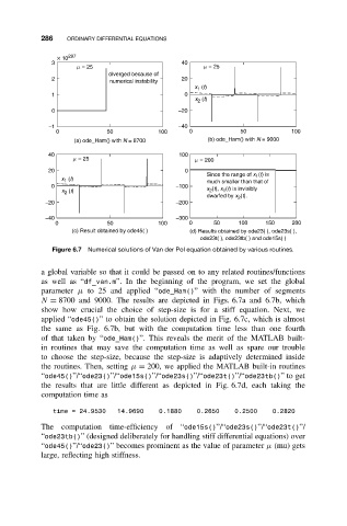
Figure 6.7 Numerical solutions of Van der Pol equation obtained by various routines.
a global variable so that it could be passed on to any related routines/functions
as well as “df_van.m”. In the beginning of the program, we set the global
parameter µ to 25 and applied “ode_Ham()” with the number of segments
N = 8700 and 9000. The results are depicted in Figs. 6.7a and 6.7b, which
show how crucial the choice of step-size is for a stiff equation. Next, we
applied “ode45()” to obtain the solution depicted in Fig. 6.7c, which is almost
the same as Fig. 6.7b, but with the computation time less than one fourth
of that taken by “ode_Ham()”. This reveals the merit of the MATLAB built-
in routines that may save the computation time as well as spare our trouble
to choose the step-size, because the step-size is adaptively determined inside
the routines. Then, setting µ = 200, we applied the MATLAB built-in routines
“ode45()”/“ode23()”/“ode15s()”/“ode23s()”/“ode23t()”/“ode23tb()”to get
the results that are little different as depicted in Fig. 6.7d, each taking the
computation time as

time = 24.9530 14.9690 0.1880 0.2650 0.2500 0.2820
The computation time-efficiency of “ode15s()”/“ode23s()”/“ode23t()”/
“ode23tb()” (designed deliberately for handling stiff differential equations) over
“ode45()”/“ode23()” becomes prominent as the value of parameter µ (mu) gets
large, reflecting high stiffness.