Page 301 - Applied Numerical Methods Using MATLAB

290 ORDINARY DIFFERENTIAL EQUATIONS
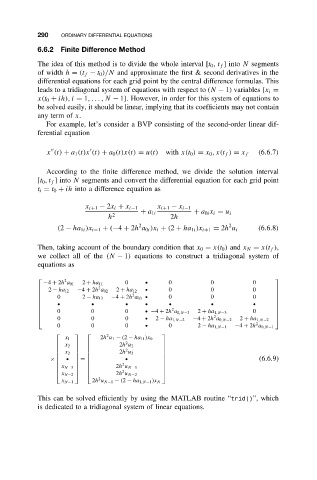
6.6.2 Finite Difference Method

The idea of this method is to divide the whole interval [t 0 , t f ]into N segments
of width h = (t f − t 0 )/N and approximate the first & second derivatives in the
differential equations for each grid point by the central difference formulas. This
leads to a tridiagonal system of equations with respect to (N − 1) variables {x i =
x(t 0 + ih), i = 1,...,N − 1}. However, in order for this system of equations to
be solved easily, it should be linear, implying that its coefficients may not contain
any term of x.
For example, let’s consider a BVP consisting of the second-order linear dif-
ferential equation

x (t) + a 1 (t)x (t) + a 0 (t)x(t) = u(t) with x(t 0 ) = x 0 ,x(t f ) = x f (6.6.7)

According to the finite difference method, we divide the solution interval
[t 0 ,t f ]into N segments and convert the differential equation for each grid point
t i = t 0 + ih into a difference equation as

x i+1 − 2x i + x i−1 x i+1 − x i−1
+ a 1i + a 0i x i = u i
h 2 2h
2 2
(2 − ha 1i )x i−1 + (−4 + 2h a 0i )x i + (2 + ha 1i )x i+1 = 2h u i (6.6.8)
Then, taking account of the boundary condition that x 0 = x(t 0 ) and x N = x(t f ),
we collect all of the (N − 1) equations to construct a tridiagonal system of
equations as

2
 
−4 + 2h a 01 2 + ha 11 0 ž 0 0 0
2
 2 − ha 12 −4 + 2h a 02 2 + ha 12 ž 0 0 0 
 2 
0 −4 + 2h a 03 ž 0 0 0
 2 − ha 13 
 
ž ž ž ž ž ž ž
 
 2 
0 0 0 0
 ž −4 + 2h a 0,N−3 2 + ha 1,N−3 
 2 
0 0 0 ž
 2 − ha 1,N−2 −4 + 2h a 0,N−2 2 + ha 1,N−2 
2
0 0 0 ž 0 2 − ha 1,N−1 −4 + 2h a 0,N−1
2
   
x 1 2h u 1 − (2 − ha 11 )x 0
2
2h u 2
  
  
2
 x 2 
2h u 3
  
 x 2 
  
×  ž  =  ž  (6.6.9)
   
x 2
   2h u N−3 
 N−3   
2
 x N−2   2h u N−2 
2
x N−1 2h u N−1 − (2 − ha 1,N−1 )x N
This can be solved efficiently by using the MATLAB routine “trid()”, which
is dedicated to a tridiagonal system of linear equations.