Page 302 - Applied Numerical Methods Using MATLAB

BOUNDARY VALUE PROBLEM (BVP) 291
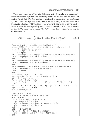
The whole procedure of the finite difference method for solving a second-order
linear differential equation with boundary conditions is cast into the MATLAB
routine “bvp2_fdf()”. This routine is designed to accept the two coefficients
a 1 and a 0 and the right-hand-side input u of Eq. (6.6.7) as its first three input
arguments, where any of those three input arguments can be given as the function
name in case the corresponding term is not a numeric value, but a function
of time t. We make the program “do_fdf” to use this routine for solving the
second-order BVP

2 2

x (t) + x (t) − x(t) = 0 with x(1) = 5,x(2) = 3 (6.6.10)
t t 2
function [t,x] = bvp2_fdf(a1,a0,u,t0,tf,x0,xf,N)
% solve BVP2: x" + a1*x’ + a0*x = u with x(t0) = x0, x(tf) = xf
% by the finite difference method
h = (tf - t0)/N; h2 = 2*h*h;
t = t0+[0:N]’*h;
if ~isnumeric(a1), a1 = a1(t(2:N)); %if a1 = name of a function of t
elseif length(a1) == 1, a1 = a1*ones(N - 1,1);
end
if ~isnumeric(a0), a0 = a0(t(2:N)); %if a0 = name of a function of t
elseif length(a0) == 1, a0 = a0*ones(N - 1,1);
end
if ~isnumeric(u), u = u(t(2:N)); %if u = name of a function of t
elseif length(u) == 1, u = u*ones(N-1,1);
else u = u(:);
end
A = zeros(N - 1,N - 1); b = h2*u;
ha = h*a1(1); A(1,1:2) = [-4 + h2*a0(1) 2 + ha];
b(1) = b(1)+(ha - 2)*x0;
for m = 2:N - 2 %Eq.(6.6.9)
ha = h*a1(m); A(m,m - 1:m + 1) = [2-ha -4 + h2*a0(m) 2 + ha];
end
ha = h*a1(N - 1); A(N - 1,N - 2:N - 1) = [2 - ha -4 + h2*a0(N - 1)];
b(N - 1) = b(N-1)-(ha+2)*xf;
x = [x0 trid(A,b)’ xf]’;
function x = trid(A,b)
% solve tridiagonal system of equations
N = size(A,2);
for m = 2:N % Upper Triangularization
tmp = A(m,m - 1)/A(m - 1,m - 1);
A(m,m) = A(m,m) -A(m - 1,m)*tmp; A(m,m - 1) = 0;
b(m,:) = b(m,:) -b(m - 1,:)*tmp;
end
x(N,:) = b(N,:)/A(N,N);
form=N-1:-1: 1% Back Substitution
x(m,:) = (b(m,:) -A(m,m + 1)*x(m + 1))/A(m,m);
end