Page 304 - Applied Numerical Methods Using MATLAB

PROBLEMS 293
ž Both methods can be modified to solve BVPs with mixed-boundary condi-
tions (see Problems 6.7 and 6.8).
ž In MATLAB 6.x, the “bvp4c()” command is available for solv-
ing linear/nonlinear BVPs with mixed-boundary conditions (see Prob-
lems 6.7–6.10).
ž The symbolic computation command “dsolve()” introduced in Section
6.5.1 can be used to solve a BVP so long as the differential equation is lin-
ear, that is, its coefficients may depend on time t, but not on the (unknown)
dependent variable x(t).
ž The usages of “bvp4c()”and “dsolve()” are illustrated in the program
“do_fdf”, where another symbolic computation command “subs()”isused
to evaluate a symbolic expression at certain value(s) of the variable.

PROBLEMS
6.0 MATLAB Commands quiver() and quiver3() and Differential Equation
(a) Usage of quiver()
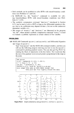
Type ‘help quiver’ into the MATLAB command window, and then you
will see the following program showing you how to use the quiver()
command for plotting gradient vectors. You can also get Fig. P6.0.1 by
running the block of statements in the box below. Try it and note that
the size of the gradient vector at each point is proportional to the slope at
the point.

%do_quiver
[x,y] = meshgrid(-2:.5:2,-1:.25:1);
z = x.*exp(-x.^2 - y.^2);
[px,py] = gradient(z,.5,.25);
contour(x,y,z), hold on, quiver(x,y,px,py)
axis image %the same as AXIS EQUAL except that
%the plot box fits tightly around the data

1

0.5

0

−0.5

−1
−2 −1.5 −1 −0.5 0 0.5 1 1.5 2
Figure P6.0.1 Graphs obtained by using gradient(), contour(), quiver().