Page 300 - Applied Numerical Methods Using MATLAB

BOUNDARY VALUE PROBLEM (BVP) 289

The solution x(t) and its derivative x (t) are known as
1 2t 2

x(t) = and x (t) = = 2tx (t) (6.6.4)
2 2
4 − t 2 (4 − t )
Note that this second-order differential equation can be written in the form of
state equation as

x (t) x 2 (t) x 1 (0) x 0 = 1/4

1
= 2 with =

x (t) 2x (t) + 4tx 1 (t)x 2 (t) x 2 (1) x f = 1/3
2 1
(6.6.5)
In order to apply the shooting method, we set the initial guess of x 2 (0) =

x (0) to
x f − x 0
dx0[1] = x 2 (0) = (6.6.6)
t f − t 0
and solve the state equation with the initial condition [x 1 (0)x 2 (0) = dx0[1]].
Then, depending on the sign of the difference e(1) between the final value x 1 (1)
of the solution and the target final value x f , we make the next guess dx0[2]
larger/smaller than the initial guess dx0[1] and solve the state equation again
with the initial condition [x 1 (0)dx0[2]]. We can start up the secant method
with the two initial values dx0[1] and dx0[2] and repeat the iteration until the
difference (error) e(k) becomes sufficiently small. For this job, we compose
the MATLAB program “do_shoot.m”, which uses the routine “bvp2_shoot()”
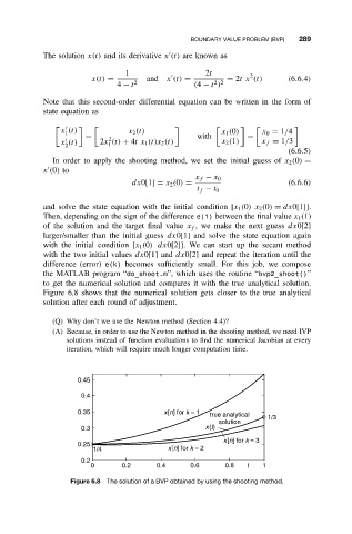
to get the numerical solution and compares it with the true analytical solution.
Figure 6.8 shows that the numerical solution gets closer to the true analytical
solution after each round of adjustment.

(Q) Why don’t we use the Newton method (Section 4.4)?
(A) Because, in order to use the Newton method in the shooting method, we need IVP
solutions instead of function evaluations to find the numerical Jacobian at every
iteration, which will require much longer computation time.

0.45
0.4

0.35 x[n] for k = 1 true analytical
solution 1/3
0.3 x(t)
x[n] for k = 3
0.25
1/4 x[n] for k = 2
0.2
0 0.2 0.4 0.6 0.8 t 1

Figure 6.8 The solution of a BVP obtained by using the shooting method.