Page 306 - Applied Numerical Methods Using MATLAB

PROBLEMS 295
1
1
× × × × × × × × × × ×× × × × ×× × × 0.5 × × × × × × × × × × × × × × × × × × × × × × × × × ×
0.8 × × + + + + + + + + + + + + + + + + + + + + + + + + + + + + + +
0.6 × × × × × × × 0 × × × + + +
+
+
+
+
+
0.4 × × × × × × × × × × × × + + +
+
0.2 × × × × × −0.5 × × × ×
0× × −1 × ×
0 0.5 1 1.5 2 0.5 1 1.5 2
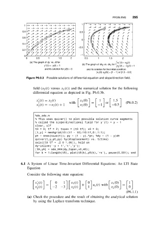
(a) The graph of dy vs. dt for x 1 ′(t) = x 2 (t)
(b) The graph of dx 2 vs. dx 1 for
y ′(t) = −y(t) + 1 x 2 ′(t) = −x 2 (t) + 1
and its solution for y(0) = 0 and its solution for the initial condition
[x 1 (0) x 2 (0)] = [1 − 1] or [1.5 − 0.5]
Figure P6.0.3 Possible solutions of differential equation and slope/direction field.
field (x 2 (t) versus x 1 (t)) and the numerical solution for the following
differential equation as depicted in Fig. P6.0.3b.

x (t) = x 2 (t) x 1 (0) 1 1.5

1 with = or (P6.0.2)
x (t) =−x 2 (t) + 1 x 2 (0) −1 −0.5

2
%do_ode.m
% This uses quiver() to plot possible solution curve segments
% called the slope/directional field for y’(t) + y = 1
clear, clf
t0 = 0; tf = 2; tspan = [t0 tf]; x0 = 0;
[t,y] = meshgrid(t0:(tf - t0)/10:tf,0:.1:1);
pt = ones(size(t)); py = (1 - y).*pt; %dy = (1 - y)dt
quiver(t,y,pt,py) %y(displacement) vs. t(time)
axis([t0 tf + .2 0 1.05]), hold on
dy=inline(’-y + 1’,’t’,’y’);
[tR,yR] = ode_RK4(dy,tspan,x0,40);
for k = 1:length(tR), plot(tR(k),yR(k),’rx’), pause(0.001); end

6.1 A System of Linear Time-Invariant Differential Equations: An LTI State
Equation

Consider the following state equation:

x (t) 0 1 x 1 (t) 0 x 1 (0) 1
1 = + u s (t) with =

x (t) −2 −3 x 2 (t) 1 x 2 (0) 0
2
(P6.1.1)
(a) Check the procedure and the result of obtaining the analytical solution
by using the Laplace transform technique.