Page 310 - Applied Numerical Methods Using MATLAB

PROBLEMS 299
R = 100[Ω] C = 10[mF ]
1
1

+ R = C =
v(t) = t [V ] i (t) 2 i (t) 2
1
2
− 1[kΩ] 10[mF]

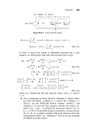
Figure P6.3.3 A two-mesh RC circuit.

1 t
R 1 i 1 (t) + i 1 (τ) dτ + R 2 (i 1 (t) − i 2 (t)) = v(t) = t
C 1 −∞
1 t
R 2 (i 2 (t) − i 1 (t)) + i 2 (τ) dτ = 0 (P6.3.7a)
C 2
−∞
In order to convert this system of differential equations into a state
equation, we differentiate both sides and rearrange them to get

di 1 (t) di 2 (t) 1 dv(t)
(R 1 + R 2 ) − R 2 + i 1 (t) = = 1
dt dt C 1 dt
di 1 (t) di 2 (t) 1
−R 2 + R 2 + i 2 (t) = 0 (P6.3.7b)
dt dt C 2

R 1 + R 2 −R 2 i (t) 1 − i 1 (t)/C 1
1 = (P6.3.7c)

−R 2 R 2 i (t) −i 2 (t)/C 2
2
−1
i (t) R 1 + R 2 −R 2 1 − i 1 (t)/C 1
1 = with G i = 1/R i

i (t) −R 2 R 2 −i 2 (t)/C 2
2

−G 1 /C 1 −G 1 /C 2 i 1 (t) G 1
= + u s (t)
−G 1 /C 1 −(G 1 + G 2 )/C 2 i 2 (t) G 1
(P6.3.7d)
where u s (t) denotes the unit step function whose value is 1 (one) ∀
t ≥ 0.
(i) After constructing an M-file function “df6p03g.m” which defines
Eq. (P6.3.7d) with R 1 = 100[ ], C 1 = 10[µF], R 2 = 1[k ], C 2 =
10[µF], use the MATLAB built-in routines “ode45()”and
“ode23s()” to solve the state equation with the zero initial con-
dition i 1 (0) = i 2 (0) = 0 and plot the numerical solution i 2 (t) for
0 ≤ t ≤ 0.05 s. For possible change of parameters, you may declare
R 1 , C 1 , R 2 , C 2 as global variables both in the function and in the
main program named, say, “nm6p03g.m”. Do you see any symptom
of stiffness from the results?