Page 291 - Applied Numerical Methods Using MATLAB

280 ORDINARY DIFFERENTIAL EQUATIONS
1.5

1
x (t)
1
0.5

0 x (t)
2

−0.5

−1
0 0.5 1 1.5 2
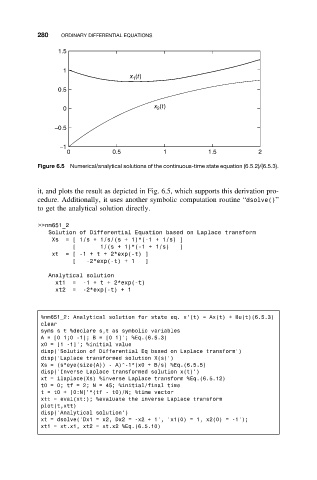
Figure 6.5 Numerical/analytical solutions of the continuous-time state equation (6.5.2)/(6.5.3).

it, and plots the result as depicted in Fig. 6.5, which supports this derivation pro-
cedure. Additionally, it uses another symbolic computation routine “dsolve()”
to get the analytical solution directly.

>>nm651_2
Solution of Differential Equation based on Laplace transform
Xs = [ 1/s + 1/s/(s + 1)*(-1 + 1/s) ]
[ 1/(s + 1)*(-1 + 1/s) ]
xt =[-1+t+ 2*exp(-t) ]
[ -2*exp(-t) + 1 ]
Analytical solution
xt1 = -1+t+ 2*exp(-t)
xt2 = -2*exp(-t) + 1

%nm651_2: Analytical solution for state eq. x’(t) = Ax(t) + Bu(t)(6.5.3)
clear
syms s t %declare s,t as symbolic variables
A=[01;0 -1];B=[0 1]’; %Eq.(6.5.3)
x0 = [1 -1]’; %initial value
disp(’Solution of Differential Eq based on Laplace transform’)
disp(’Laplace transformed solution X(s)’)
Xs = (s*eye(size(A)) - A)^-1*(x0 + B/s) %Eq.(6.5.5)
disp(’Inverse Laplace transformed solution x(t)’)
xt = ilaplace(Xs) %inverse Laplace transform %Eq.(6.5.12)
t0 = 0; tf = 2; N = 45; %initial/final time
t = t0 + [0:N]’*(tf - t0)/N; %time vector
xtt = eval(xt:); %evaluate the inverse Laplace transform
plot(t,xtt)
disp(’Analytical solution’)
xt = dsolve(’Dx1 = x2, Dx2 = -x2 + 1’, ’x1(0) = 1, x2(0) = -1’);
xt1 = xt.x1, xt2 = xt.x2 %Eq.(6.5.10)