Page 287 - Applied Numerical Methods Using MATLAB

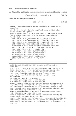
276 ORDINARY DIFFERENTIAL EQUATIONS
we obtained by applying the same routines to solve another differential equation

y (t) = y(t) + 1 with y(0) = 0 (6.4.11)
where the true analytical solution is
t
y(t) = e − 1 (6.4.12)

%nm643_1: RK4/Adams/Hamming method to solve a differential eq
clear, clf
t0 = 0; tf = 10; y0 = 0; %starting/final time, initial value
N = 50; %number of segments
df643 = inline(’-y+1’,’t’,’y’); %differential equation to solve
f643 = inline(’1-exp(-t)’,’t’); %true analytical solution
for KC = 0:1
tic, [t1,yR] = ode_RK4(df643,[t0 tf],y0,N); tR = toc
tic, [t1,yA] = ode_ABM(df643,[t0 tf],y0,N,KC); tA = toc
tic, [t1,yH] = ode_Ham(df643,[t0 tf],y0,N,KC); tH = toc
yt1 = f643(t1); %true analytical solution to plot
subplot(221 + KC*2) %plot analytical/numerical solutions
plot(t1,yt1,’k’, t1,yR,’k’, t1,yA,’k--’, t1,yH,’k:’)
tmp = abs(yt1)+eps; l_t1 = length(t1);
eR = abs(yR - yt1)./tmp; e_R=norm(eR)/lt1
eA = abs(yA - yt1)./tmp; e_A=norm(eA)/lt1
eH = abs(yH - yt1)./tmp; e_H=norm(eH)/lt1
subplot(222 + KC*2) %plot relative errors
plot(t1,eR,’k’, t1,eA,’k--’, t1, eH,’k:’)
end

%nm643_2: ode23()/ode45()/ode113() to solve a differential eq
clear, clf
t0 = 0; tf = 10; y0 = 0; N = 50; %starting/final time, initial value
df643 = inline(’y + 1’,’t’,’y’); %differential equation to solve
f643 = inline(’exp(t) - 1’,’t’); %true analytical solution
tic, [t1,yR] = ode_RK4(df643,[t0 tf],y0,N); time(1) = toc;
tic, [t1,yA] = ode_ABM(df643,[t0 tf],y0,N); time(2) = toc;
yt1 = f643(t1);
tmp = abs(yt1)+ eps; l_t1 = length(t1);
eR = abs(yR-yt1)./tmp; err(1) = norm(eR)/l_t1;
eA = abs(yA-yt1)./tmp; err(2) = norm(eA)/l_t1;
options = odeset(’RelTol’,1e-4); %set the tolerance of relative error
tic, [t23,yode23] = ode23(df643,[t0 tf],y0,options); time(3) = toc;
tic, [t45,yode45] = ode45(df643,[t0 tf],y0,options); time(4) = toc;
tic, [t113,yode113] = ode113(df643,[t0 tf],y0,options); time(5) = toc;
yt23 = f643(t23); tmp = abs(yt23) + eps;
eode23 = abs(yode23-yt23)./tmp; err(3) = norm(eode23)/length(t23);
yt45 = f643(t45); tmp = abs(yt45) + eps;
eode45 = abs(yode45 - yt45)./tmp; err(4) = norm(eode45)/length(t45);
yt113 = f643(t113); tmp = abs(yt113) + eps;
eode113 = abs(yode113 - yt113)./tmp; err(5) = norm(eode113)/length(t113);
subplot(221), plot(t23,yode23,’k’, t45,yode45,’b’, t113,yode113,’r’)
subplot(222), plot(t23,eode23,’k’, t45,eode45,’b--’, t113,eode113,’r:’)
err, time