Page 283 - Applied Numerical Methods Using MATLAB

272 ORDINARY DIFFERENTIAL EQUATIONS
We still cannot use these formulas to estimate the predictor/corrector errors, since
K is unknown. But, from the difference between these two formulas
270 270 270
∼ 5
E P,k+1 − E C,k+1 = c k+1 − p k+1 = Kh ≡ E P,k+1 ≡− E C,k+1
720 251 19
(6.4.5)
we can get the practical formulas for estimating the errors as
251
∼
E P,k+1 = y k+1 − p k+1 = (c k+1 − p k+1 ) (6.4.6a)
270
19
∼
E C,k+1 = y k+1 − c k+1 = − (c k+1 − p k+1 ) (6.4.6b)
270
These formulas give us rough estimates of how close the predicted/corrected
values are to the true value and so can be used to improve them as well as to
adjust the step-size.

251
p k+1 → p k+1 + (c k − p k ) ⇒ m k+1 (6.4.7a)
270
19
c k+1 → c k+1 − (c k+1 − p k+1 ) ⇒ y k+1 (6.4.7b)
270
These modification formulas are expected to reward our efforts that we have
made to derive them.
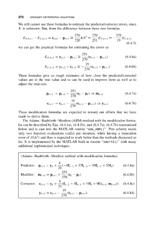
The Adams–Bashforth–Moulton (ABM) method with the modification formu-
las can be described by Eqs. (6.4.1a), (6.4.1b), and (6.4.7a), (6.4.7b) summarized
below and is cast into the MATLAB routine “ode_ABM()”. This scheme needs
only two function evaluations (calls) per iteration, while having a truncation
5
error of O(h ) and thus is expected to work better than the methods discussed so
far. It is implemented by the MATLAB built-in routine “ode113()” with many
additional sophisticated techniques.

Adams–Bashforth–Moulton method with modification formulas
h
Predictor: p k+1 = y k + (−9f k−3 + 37f k−2 − 59f k−1 + 55f k ) (6.4.8a)
24
251
Modifier: m k+1 = p k+1 + (c k − p k ) (6.4.8b)
270
h
Corrector: c k+1 = y k + (f k−2 − 5f k−1 + 19f k + 9f(t k+1 , m k+1 )) (6.4.8c)
24
19
y k+1 = c k+1 − (c k+1 − p k+1 ) (6.4.8d)
270